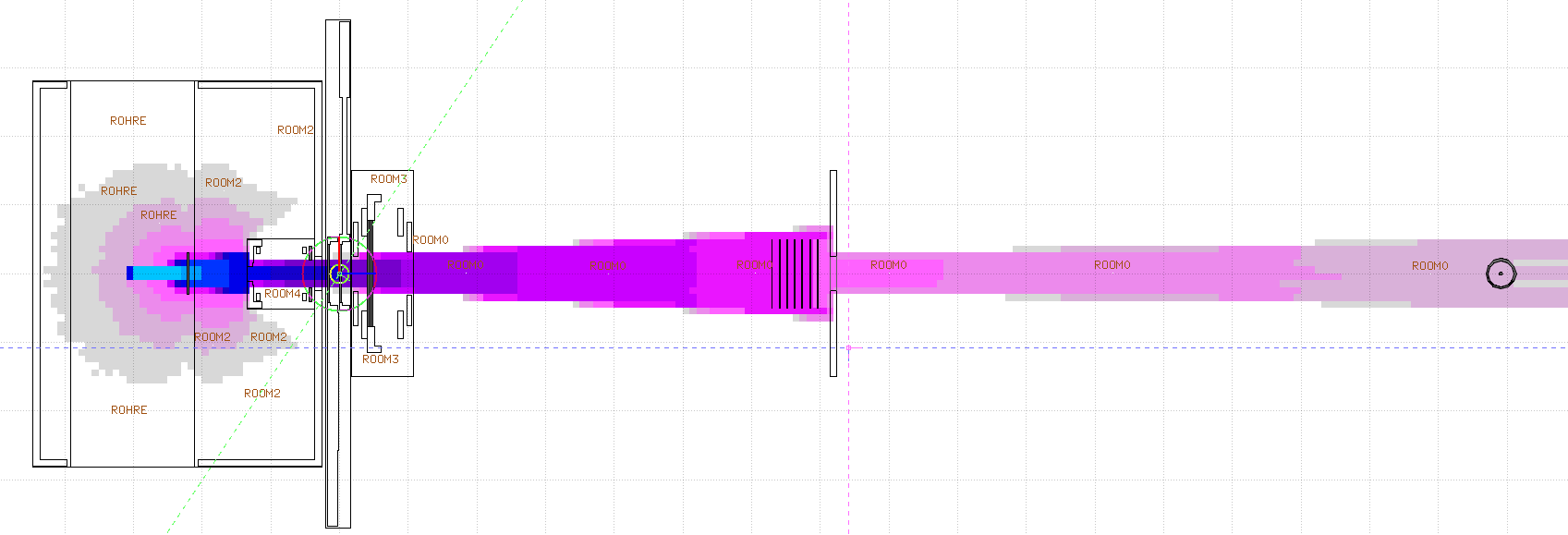
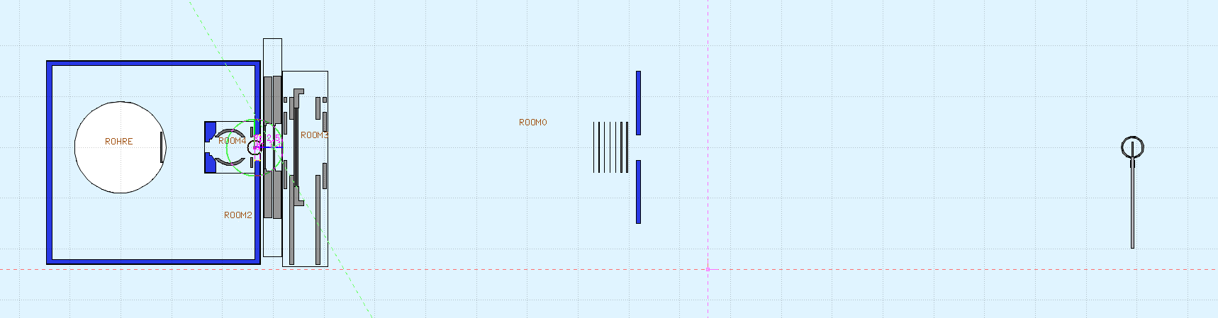
I’m trying to simulate the X-ray beamline in our lab, mainly to do some absorption calculations /determination of half-value layers. The distance between source and detector is 2 m and the detector has a sensitive volume of approx. 28 cc.
Half way between the focal spot and the detector (around 1 m distance) I’m placing aluminium absorbers of different thicknesses. Please, see attached figures.
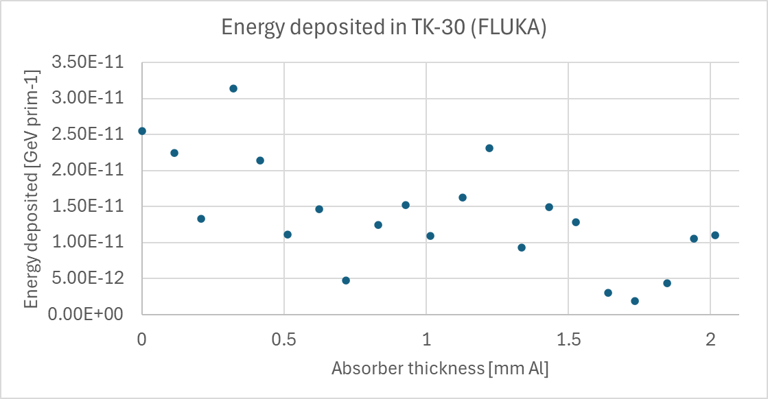
The sensitive volume is so small, that after running 1e8 primaries for several hours, the values of energy deposited estimated with a USRBIN card in the scoring region while adding absorbers fluctuate a lot (see plot attached). Therefore, I figured I’d use some kind of biasing. I started with the easiest one, namely using a region importance BIASING card in each of the absorber plates, increasing the importance of photons and electrons in a power-of-two sequence. According to what I read in Biasing in an air tunnel this should be appropriate for my problem.
After applying the BIASING card, I obtained essentially the same results as before. What I’ve learned until now is that the biased regions should be placed next to each other, which is not my case, as the absorbers are enclosed in a bigger air region and there is about 1 cm distance between them.
I could create “air regions” between the absorbers, and use them to increase the importance as well, but then the following questions arise:
Should I continue increasing the importance until I reach the detection volume?
Should the detection volume be biased as well?
I’ve read about the problematic with the adjacent regions, which should have the same importance in case they can contribute to the results in the scoring region. Could this be potentially an issue in my approach?
Finally, is this the correct way to approach such an absorption problem?
I attach an example of input file for reference.
Thank you all in advance for any help you can provide!
Hello Federico,
I looked at your input file. The BIASING card is commented out, but if this was the biasing you applied, there are two issues with it:
1.) to give increasing weights to a series of regions, each of them requires a BIASING card with the weight.
2.) Your filters are embedded in air (actually in ROOM0). Imagine ROOM0 has weight 1 (default) and one of the filters has weight 2.What happens with the photon (splitting or russian roulette, RR) is determined at a region boundary by the ratio of the region weights. A photon would enter from ROOM0 to the filter and probably be split, because the weight in the filter region is higher. However, when leaving the filter and re-entering ROOM0, the inverse weight ratio applies and the additional photon may vanish after RR.
To avoid this from happening, you can give the air between two filters the weight of the previous filter. The same applies to the air after the filter stack and the detector. The photons should travel along a path consisting of regions with monotonously increasing weights.
Best, Thomas
Yes, some cards are commented because I want to add the filters in steps, I just uploaded one example with some of the biasing cards uncommented corresponding to those absorbers that are not “air”.
So, if I understand correctly, my initial assumption was right: starting from the first region where the biasing is introduced and continuing all the way to the final region (i.e. the scoring region), the regions must be adjacent and have increasing importance according to a power-of-two sequence. This would mean that the scoring region itself also needs to be assigned an importance. Is that correct?
In my case, this would imply defining several additional air regions between the absorbers, as well as between the filters and the detector, so that the importance can increase continuously until reaching the detector.
What about the adjacent air, i.e. the rest of the room that surrounds these biased regions? Its importance would presumably remain at 1. Could having importance-1 air directly adjacent to the biased regions cause any problems or interfere with the importance splitting or my scoring?
Thanks again for you input, it’s really appreciated.
you are right with your description. Only the air layers don’t have to get a weight increased by 2.
The power-of-two is a rule of thumb, I sometimes try to estimate the weight increase of a region from the inverse of the attenuation coefficient of a medium. To determine the “best possible region weight” you would first have to solve the transport problem, which is the aim of your simulation
As a rule, I would extend the biased region of air to more than only the size of the filters. Like this you will take into account photons back-scattered from air - not an important effect. If, however, you would simulate the propagation of photons in a water phantom, or through a shielding, then this effect cannot be neglected, it constitutes the so-called build-up for a broad beam in matter.
In addition to Thomas’ answers which well describes some critical aspects in the setup of the biasing scheme for your current study, I would like to propose you another approach which does not require any biasing technique.
I used the input file you have provided (thanks!) to do a quick simulation. After removing the SOURCE card which was interfering with the angular description of the photon beam, I have scored the current of photons entering the detector region TK30_Vol: ~2.5E-03 particle/primary reach the detector while many are lost due to the aperture of the beam and the presence of the collimator.
This implies that 1 primary out of ~400 would reach the detector itself (and possibly deposit energy), and therefore a lot of simulation time is actually spent in tracking uninteresting photons.
What I would suggest is to follow a 2-steps simulation (more details at this link) instead.
The idea would be the following:
Step 1. Starting with the 300 keV beam, the phase space of the photon reaching the aperture of the collimator is scored for the different Al thicknesses of interest.
Step 2. Starting with primary the scored photon phase space, you track them to score the energy deposition in the detector.
As usual in these two steps simulation approach, attention should be paid to the normalization of the results of the second step. More information in the link posted before.
Let me know if this could be a valuable solution to your problem,
Giuseppe
Thanks for your response and suggestion. It is indeed an interesting method, and maybe a comparison of both methodologies would be a good idea.
At some point I will need to start closing the aperture to make the field smaller (while always illuminating the complete detector), because I need to calculate the zero field size approximation (requirement of ISO 4037 for the determination of a unique half-value layer).
I need to evaluate which methodology would require less simulations and will be faster to implement.
If I find something interesting, I’ll come back to post it.