Scoring H3 and He4 in optical fiber

[xiongbp (XIONG BANGPING)]

Test.inp (3.6 KB)

Dear David,
Thank you for your help,I have another question…
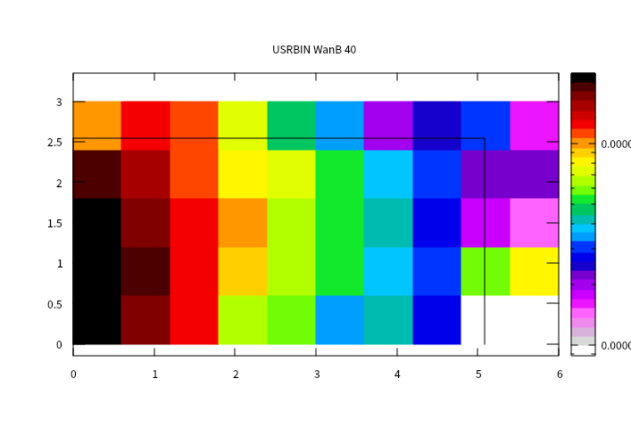
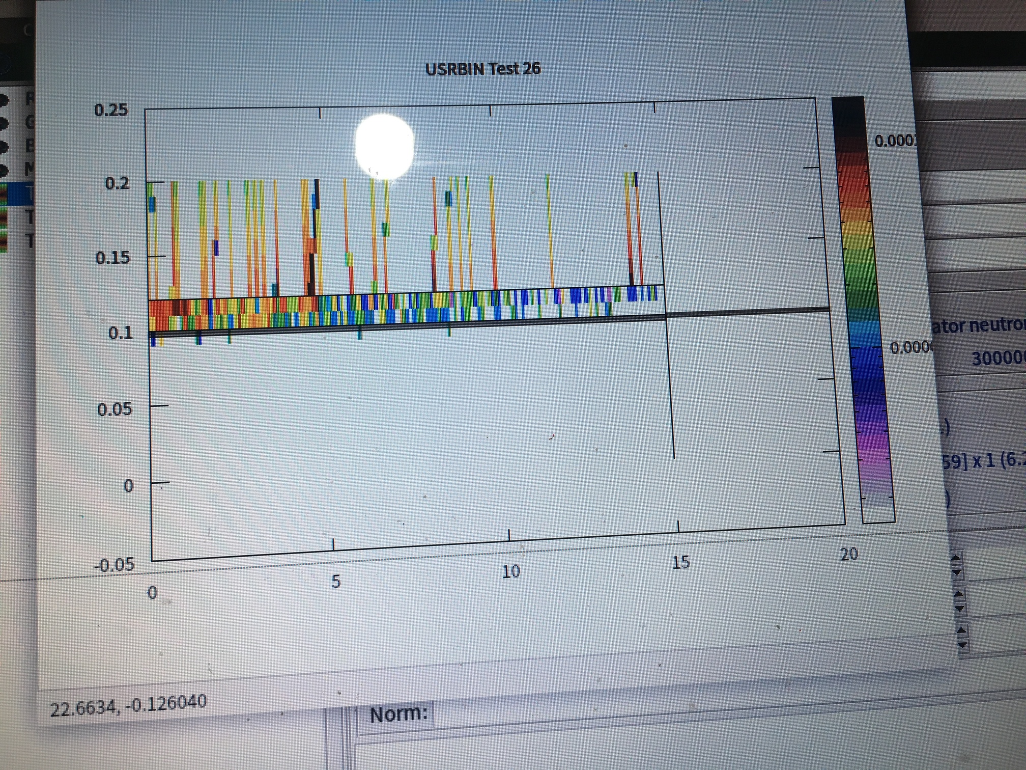
As the attachment “WanB.inp"shows,I run the file and plot,but the result is just like the attachment"WanB_40_plot”,does it caused by any software settings?

[adonadon (Andre Donadon Servelle)]

Dear Xiong,

Thanks for your question.
Could you explain me in more detail what you try to obtain
using this scoring? (What do you expect?)

Btw, I saw quickly your input ‘Test.inp’ and it has an error in the definition of the geometry.
You should define in your ‘void’ region an extra zone that could be like this:

| -plane3 +jacket

Then, if you can explain me a bit more the scoring that you defined and also the
purpose of the simulation I will try to help you as soon as possible

Best,
André

[xiongbp (XIONG BANGPING)]

Dear Andre,
1.Thank you for your remind ,I forget add a zone"|-plane3+jacket"to the region “void”;
2.I use a “wavelength shifting fiber + optical fiber” to simulate a neutron detector.

first, I want to get the relationship between the secondary particles’ counting (He-4,H-3)and the thickness of region “COAT” ;
second, I want to get the distribution of secondary particles’ fluence in region “COAT” to ensure how the thickness of “COAT” should be to get maximum optical photon.
This file has not been added to optical card, I will add it later.
Best,
Xiong

[adonadon (Andre Donadon Servelle)]

Dear Xiong,

Thanks for clarifying the problem.

For the first point:

One way to compare the number of He-4 + H4-3 with different thickness could be using the card USRTRACK.
With this card you will be able to obtain the energy spectrum of a desired particles. I suggest you to read this thread:

Accessing particles data in FLUKA

Dear experts, I am new to Fluka and Flair, before i only worked with c++ packages like Geant4, Pythia8. I want to compare Geant4 and Fluka for one experiment. In Geant4 i can access all secondaries data on each step. This way i can get spectrums of particles when they leave target(i simply call function to give me particle energy on the last step before it deletes). Using flair i understood how to use USRBIN. But how can i simulate perfect detector that returns value of energy, or transverse mo…

Another option, If I understand properly and what you want is to count the number of He-4 and He-3 generated in a particular region you can use MDSTCK. It is a subroutine part of MGDRAW, that is is called every time a secondary particles is generates. With that you can calculate the number of particles generated. To use MGDRAW you can look this thread where it is explained:

Use of MGDRAW with my input file

Dear fluka Expert I am still a beginner and I want to use MGDRAW with my input file on flair. I have modified the MGDRAW file to suit my input file and expectation result but I don’t know how to connect both MGDRAW and input file together and run. Is there any specific area in the manual that explains this? I am new on how to user routine.

For the second point:
I would suggest you to use the scoring card USRBDX.
You can look the manual here (USRBDX)
So, as not be repetitive I propose you to read these other threads where you can find very well
explained how to use this card:

Accessing particles data in FLUKA - #4 by yurchenko.sv (Again, but ony last answer)
Best way to score the number of beam particles in a region - #4 by duarte.guerreiro

If I understood correctly, in your case you will need to define one USRBDX card, from region ‘COAT’, to 'JACK2, for the particle ‘OPTIPHOT’ (I suppose that It was your strategy when you defined your second USRBIN card)

Just a last comment, sometimes the plots obtained from the PLOT tab in a projection may be not so intuitive, that’s why I propose you to do the next in order to see your scoring in the GEOMETRY tab on Flair:

1. Go Geometry
2. Window on your left, subtab ‘Layers’
3. Select one of the layers that you are using ( e.g. Media)
4. Press and Usrbin
5. The usrbin window will appear and there you have to choose the .bnn file of interest ( choose also the detector)

Then, you will be able to plot your results.

Let me know if you need more help,

Best,
André

[xiongbp (XIONG BANGPING)]

1.inp (1.7 KB) Test.inp (3.8 KB)
Dear Andre,
Thank you for your patient help,I still have some questions as below:

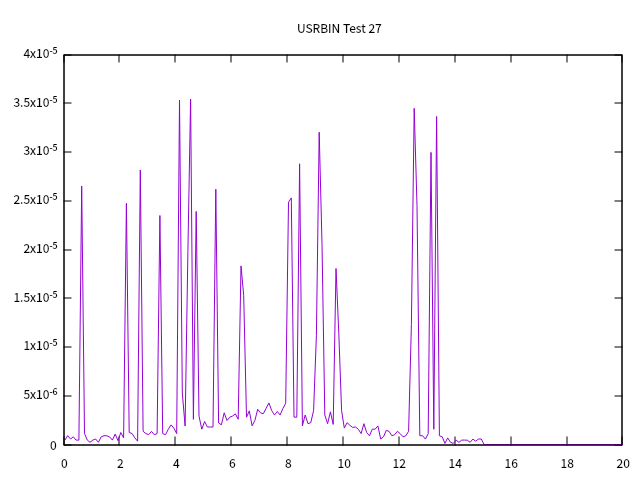
1. when I use “test.inp” to plot USRTRACK,it gave errors "line 0: all points y value undefined! ",but I do not find where is “line 0”.so I use another simple file named “1.inp” to find that USRTRACK shows a graph about energy spectrum.It’s weird that triton energy at 5e-5Gev have largest quantity below 1 and absolutely unexpected(as we know,thermal neutron react with 6LiF can not generate triton at that high energy)…Maybe I do not express my point clearly but I guess the relationship between layer thickness and number of He4+H1 may be not this card because I only care the thickness and the number of secondary particles.
2. I’m not familiar to MDSTCK,just learning now.Here I just find another question,if I want to define a radiation source at cylinder 's lateral,may I use BEAMPOS(for example x=1,y=1,z=0,cosx=0.707,cosy=0.707, but what should type set to be?)
3. I use USRBDX in the test.inp, but it have no response to plot,am I set something wrong?
4. optical photon part I will consult it later.
5. When I select one of the layers ,there is nothing difference ,so I’m not actually understand “press and usrbin”.

I use some files to learning, but the final plot and graph always unexpected, so I think there maybe some common reasons.

[adonadon (Andre Donadon Servelle)]

Dear Xiong,

Sorry for the delay in replying.

I’ve seen your files, so let’s go point by point:

1. The error ‘line 0: all points y value undefined!’ is telling basically that you do not have generation of Triton at the region ‘COAT’ in the range of energies that you defined. Anyway, then would be better if you use for this the subroutine MDSTCK, where you can calculate the number of secondary particles in the region of interest.
2. Ok, let me know if you are able to use MDSTCK, otherwise we can discuss it. For the source yes, with that card you can define the position of the primary particles (neutrons in your case), and the cos angle. But, in your particular case, you selected an isotropic source, then being isotropic the info that you provide for the angle in BEAMPOS is meaningless, but the position of your source is used.
   What do you really need for your source? For the moment I leave you here a presentation about this topic.
3. USRBDX, in your file, is defined from region ‘COAT’ to region ‘COAT’. Actually this card is used to obtain the boundary crossing fluence which it is not what you are looking for (I think I misunderstood what you needed) If you need to get the fluence in the region ‘COAT’ you should use the USRBIN card.
   The problem that your are facing is that there is no generation of Triton, that is why your are not getting anything in the USRBIN result.
4. Ok!
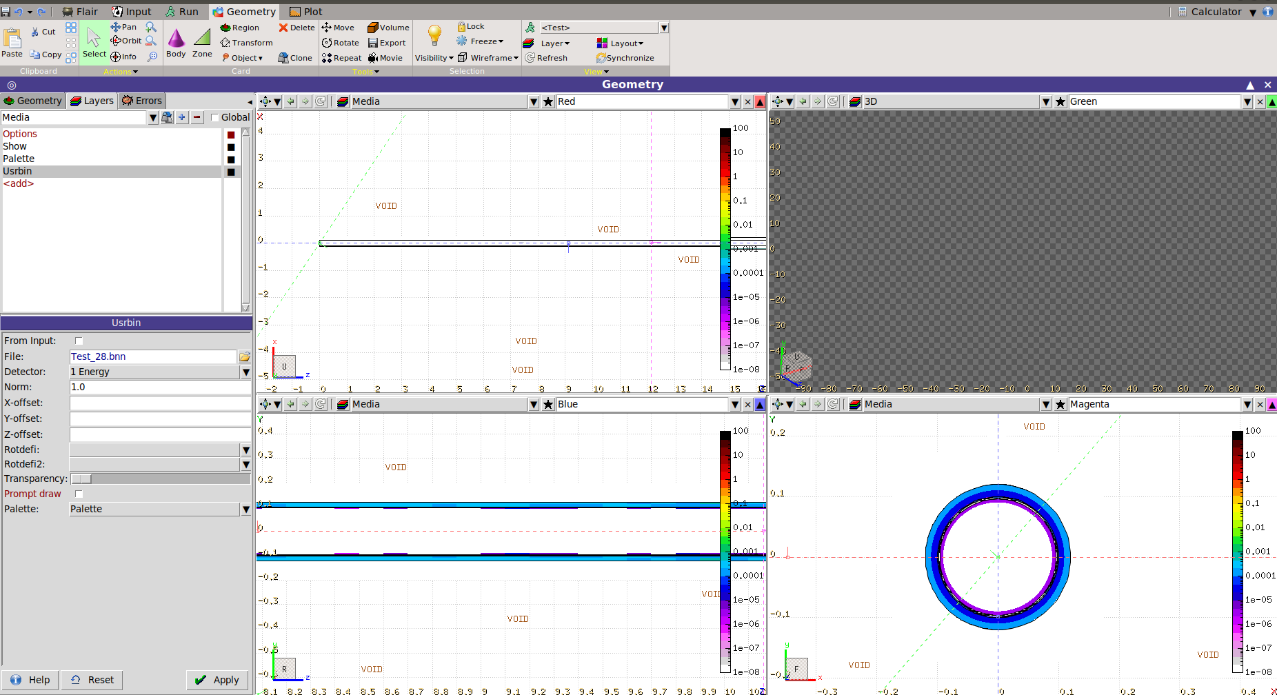
5. I was saying that… when you press "add>’ you can select ‘Usrbin’. Then you will see a new window below this one named ‘Usrbin’. There you can choose the result you obtained using Usrbin and plot it on the geometry

An extra feature that is quite useful to see your simulations is simply plot the track of your particles.
The routine to get that is MGDRAW. It is easy to use:

Just adding the card USERDUMP with the following values:

It should work. And then doing the same steps that I told for the USRBIN case but doing it for USERDUMP you will be able to see the tracks.

I hope It can help,
Have a nice weekend!

André

[xiongbp (XIONG BANGPING)]

Test.inp (3.8 KB)
Dear André,
Thank you for your reply.

1. I want a point-like and isotropic thermal neutron source,so the settings of BEAM and BEAMPOS of the attachment is ok?
2. The region “COAT” have mixed with material “6LiF”,it is weird that there is no generation of triton.
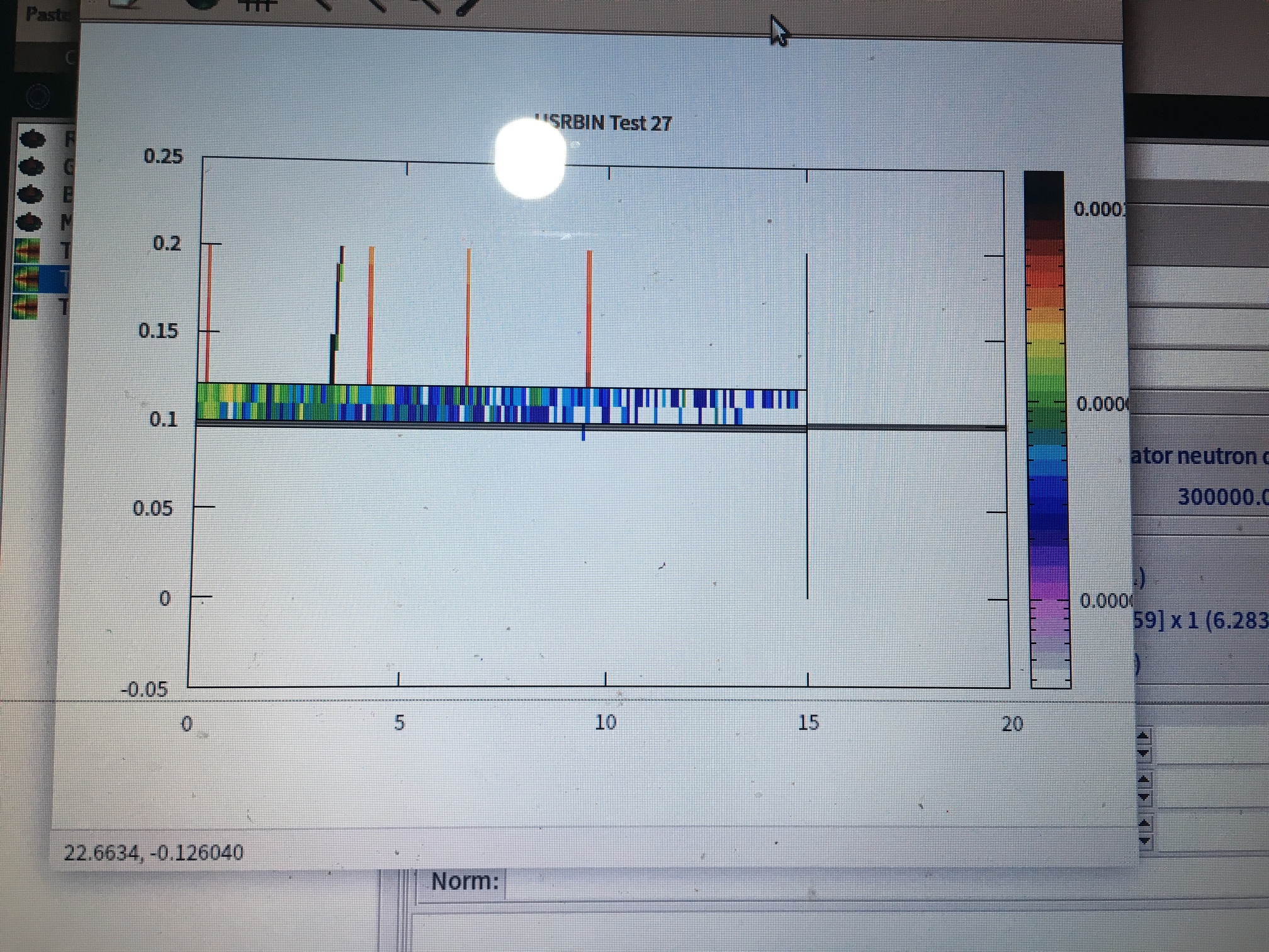
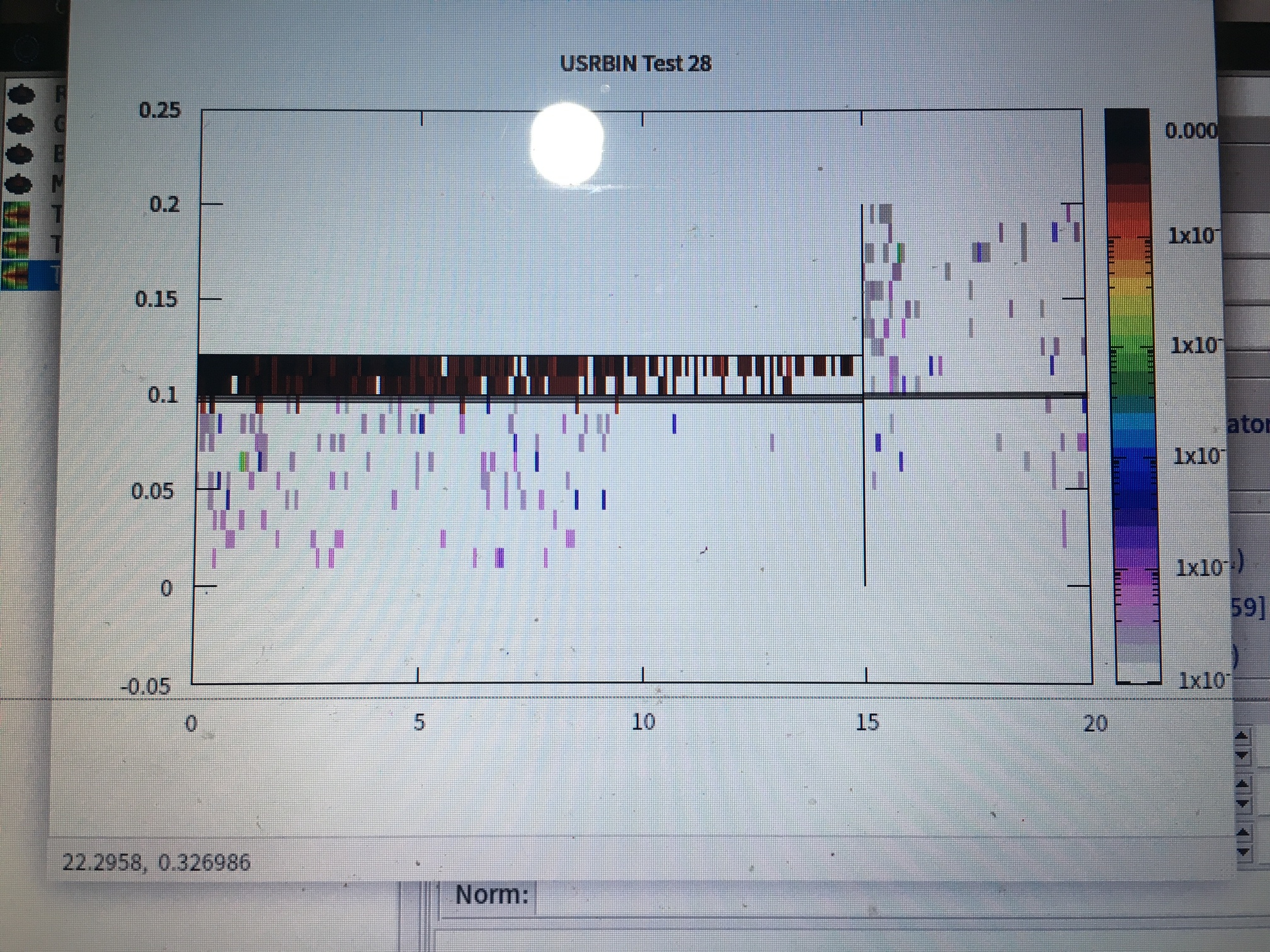
3. I have use USRBIN to plot the distribution of He-4 ,triton and energy at the region “COAT”,but the result is something strange,I do not know the reason.
4. press “add” and select “USRBIN”…but there is nothing different,please see the attachment.

[adonadon (Andre Donadon Servelle)]

Dear Xiong,

1. Yep, It is perfect. You chose the isotropic source with BEAM (which is perfect) and then you can decide with BEAMPOS only the position of the point-like source. Then, what you did is ok.
2. There is, you will see it better doing the step 4 properly (I will attach a few pictures and send you a new input file)
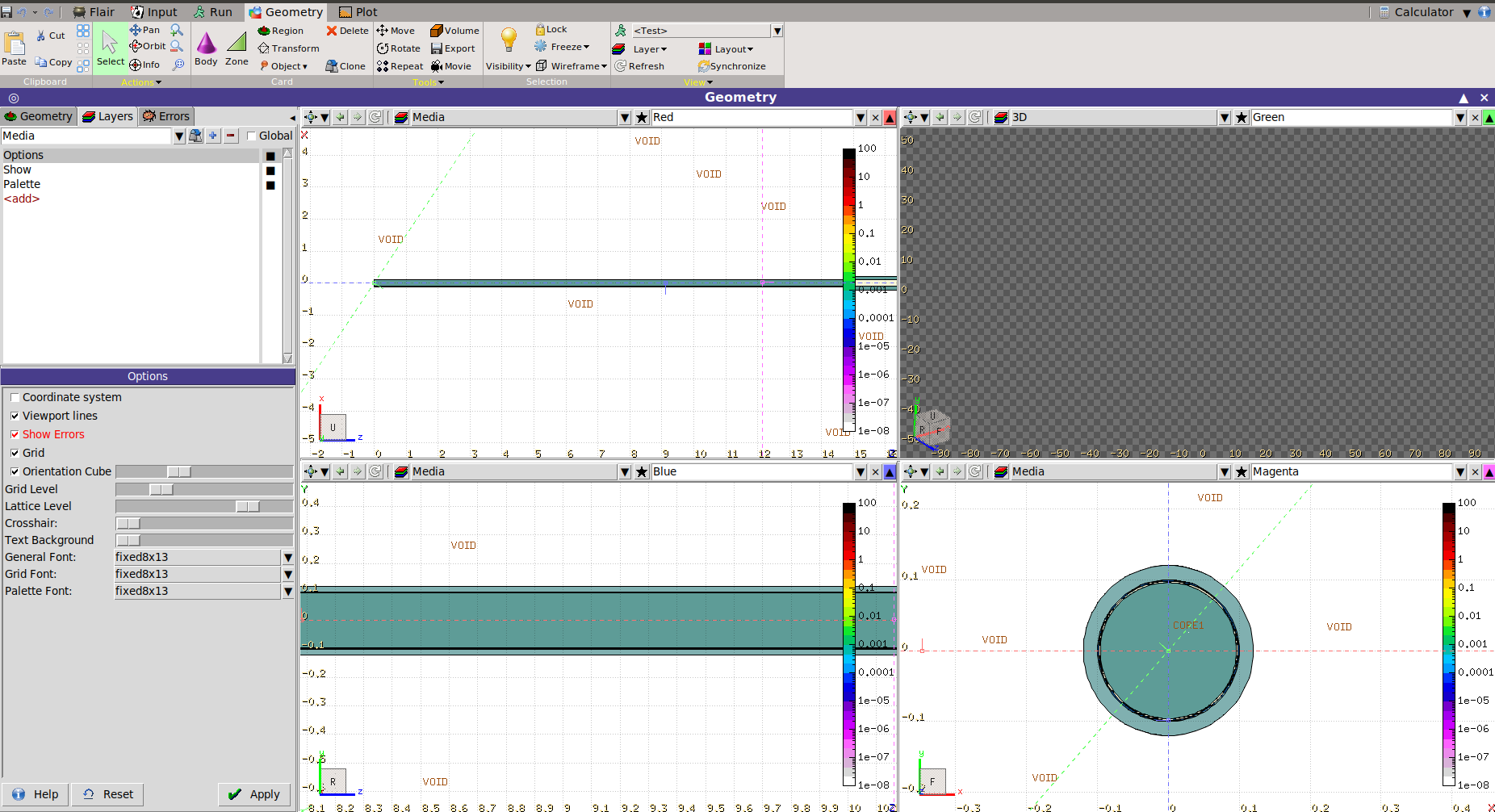
3. It is due to the projection used for the plot. There you can see the fluence of 4-Helium in your region (which is ‘COAT’+'CORE1+ part of void around these regions)
4. Look that the layer where you are defining the USRBIN is in ‘Borders’ and in the Geometry Viewer you are display ‘3D’. You have to change it to ‘Borders’ as well.
   Let see it for the ‘media’ layer case:
   
   
   
   
   
   
   
   

And there you can see the energy deposited by all the particles in that region.
I attach here the input:

Test.inp (3.8 KB)

Last comment. You can also plot fluence and energy deposited in 1D (Histograms). I consider it would be useful for your study. To do this you have to go the tab ‘Plot’, choose one of your scorings and on the right you will see ‘Type: 2D projection’. There you can change for many projections in 1D, which could be a better plot in your case that the 2D.

Cheers,
André

[xiongbp (XIONG BANGPING)]

Dear André,
Thank you for your reply.
I know the use of layers,it show me the distribution of files like “.bnn” on geometry directly.I still have some questions below.

1. In the geometry viewer,why the secondary particles’ distribution discontinuity(colour block lightly and discontinuity ),is my model’s reason?
2. I change to projections in1D,because the USRBIN is R-phi-Z,the x-axis is the Zmin to Zmax where I defined at USRBIN,but the y-axis is not R I defined at USRBIN,how the graph demonstrate the relationship of R/Z/Fluence
   
3. I have use USRDUMP,so should I add corresponding user routine?
   Best,
   Xiong

[adonadon (Andre Donadon Servelle)]

Dear Xiong,

Sorry, Could you please repeat the first two questions?, I don’t think I understand what you mean.
3. Using the USERDUMP card it will call the default MGDRAW and after the simulation you will get an output file (*dump) that you can plot in the Geometry Viewer in the same way as you did for USRBIN. I leave here the input with that:

Test.inp (3.8 KB)

Cheers,
André

[xiongbp (XIONG BANGPING)]

Dear André,
I think I have understand the first two question.
1.it is actually the model’s reason,because the production of secondary particles is limited.so the colour at the defined region of geometry tab does not look smoothly,just like colour block(at your third picture,orientation R,enlarge it and some colour like purple block).
2.The second maybe not a question,it is my misunderstand.because I changed it to 1D projection,so it just shows the relationship between the fiber length and He-4 fluence, independence of the radius.
3.ok,I understand the USERDUMP.

[xiongbp (XIONG BANGPING)]

Dear André,
I have understand this topic ,thank you for your kindly help.