Biasing strategy based on directing particle weights

[koen.de.mare]

Dear Fluka experts,

On learning that user biassing through usimbs can use the current weight of the particle in calculating the splitting or russian-rouletting ratio, I had an idea on how to use this for biasing and wanted to check if this is a sensible and safe approach. In short, the idea is to assign a narrow weight band to every position in space and to split or russian-roulette particles accordingly.

To describe/illustrate this I’ll be showing plots of this strategy with a really simple toy model of an 1 MeV photon beam incident on a lead slab.

weight-steering-biassing-main.zip (7.0 KB)

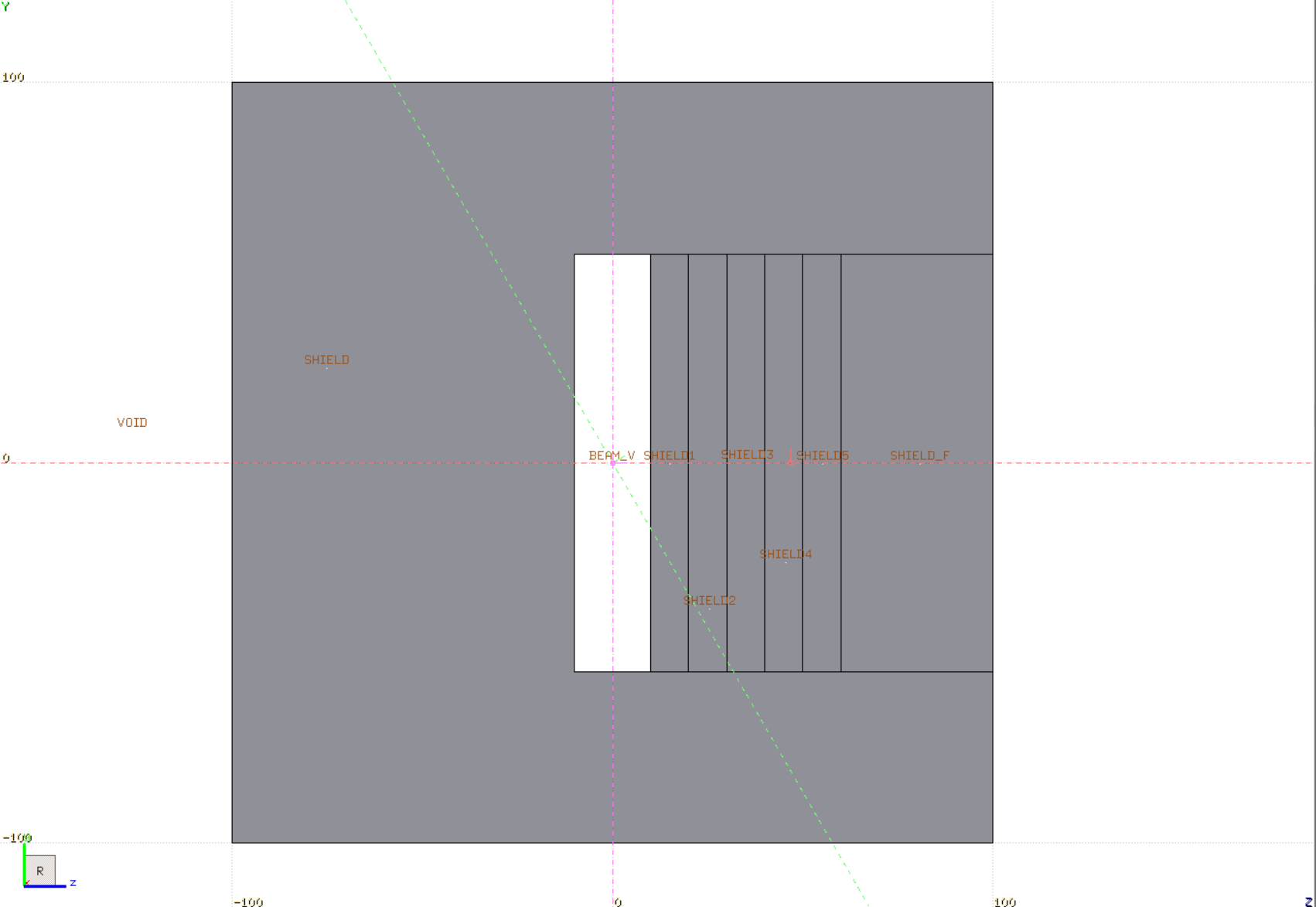
The beam is at x=y=z=0, and is a r=50 cm beam facing positive z, giving a uniform radiation distribution in the lead at z>10 cm.

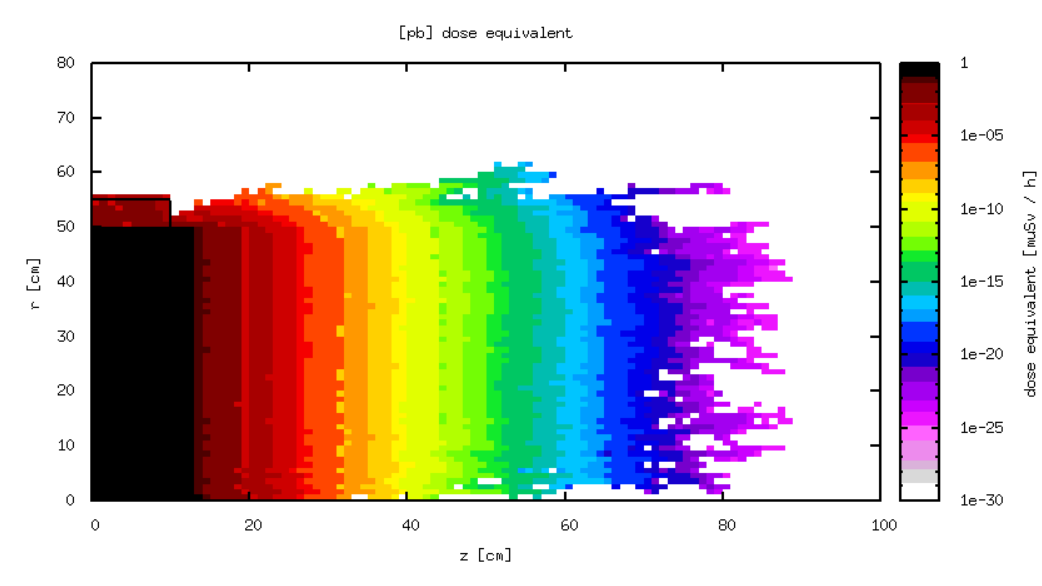
The goal is to calculate the dose-equivalent over distance, which (with biasing) will give something like:

My intuition on biasing through shielding is that performance is best when the number of simulated particles entering the shielding is approximately the same as the number of particles leaving the shielding (neglecting any weight variations). To tune this, I’ve been abusing USERWEIG/fluscw to score the fluence of particles that are simulated in some region. In this model, with biasing this gives plots such as:

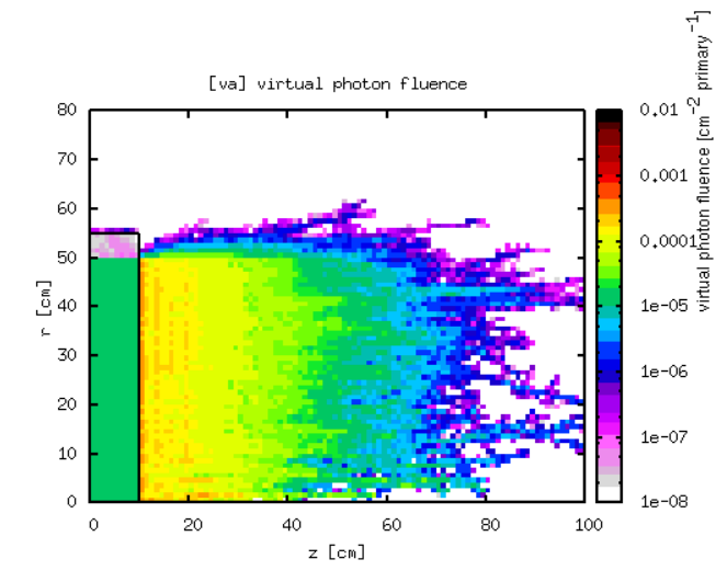
Note that this just spans six orders of magnitude (sensible as about 1e5 primaries were simulated), whereas the dose-equivelent generated with the same biassing and same number of primaries spans 25 orders of magnitude, indicating that the biasing is helping.

Now getting to the biassing itself: without biassing the decrease in dose-equivelent is largely caused by a decrease in simulated particles. It is better to instead decrease the weight of simulated particles, making the decrease in simulated particles less strong. This leads to the idea of some “target weight” at every position.

With usimbs being able to use the coordinates of the particle and the current weight of the particle, we can calculate the target weight at its new position and compare this with the current weight to check if we should be splitting or performing russian-roulette, and set FIMP accordingly.

In this simulation, I set the target weight as an exponential decay with a 1/10 length of some 3.5 cm, which is approximately the same 1/10 length as the dose-equivalent as can be seen in the earlier dose-equivalent figure.
If the current weight of a particle is more than 4x the target weight, FIMP = 2 to split the particle in two.
If the current weight is less than 1/4x the target weight, FIMP = 0.5 to russian roulette.
This strategy should keep the weights of particles in a band near the prescribed weight-distribution, also keeping the weight variation bound to approximately a factor of 16. The usimbs code of this biasing is as follows:

      ZEND = ZTRACK(NTRACK)

*     Biasing settings
      BIASFT = 1.1d0
      BIASL = 0.14d0

*     weight starting point
      WSTART = 1d0
      BSTART = 10d0
      
*     relative weight margin
      WMARG = 4d0

*     calculate importance of the current position
      BIASIMP = BIASFT**NINT((ZEND-BSTART)/BIASL)
*     calculate the target weight at the current position
      WTARG = WSTART / BIASIMP

      IF ( WTRACK .GT. WTARG * WMARG) THEN
*        weight is too large
         FIMP = 2d0
         RETURN
      ELSE IF ( WTRACK * WMARG .LT. WTARG) THEN
*        weight is too small
         FIMP = 1d0 / 2d0
         RETURN
      ELSE
*        weight is fine
         FIMP = ONEONE
         RETURN
      END IF

Using another trick with USERWEIGH/fluscw we can plot the weights of simulated particles at various interfaces, giving:

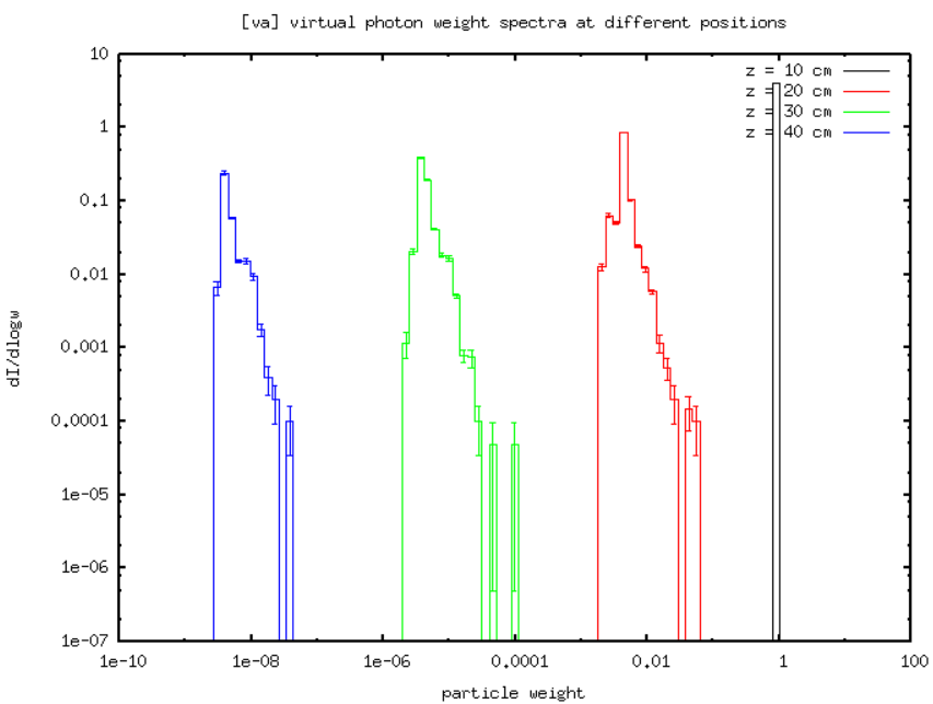
showing that indeed the current of simulated particles remains similar, but the weight is decreasing over z. The rather tight distribution of weights is also clear.

Using this biasing to score the physical dose-equivalent gives the first shown figure.

I found this strategy to be quite convenient in the first more serious project I used it in, as it by default keeps weight variation in check while not requiring too much tuning. The virtual fluence scoring makes the tuning quite straight-forward as well.

I am aware that doing in combination with lambda-biassing is somewhat risky, as lambda-biassing can cause weight fluctuations. The interaction with leading particle EMF biassing is less clear to me: while it should be safe to use I’m not sure how it affects (statistical) performance, if someone has ideas about this that would be appreciated.

I hope someone can give opinions on this being a useful strategy, if this strategy has the risk of giving misleading results or if there are different better ways of approaching usimbs biasing.

Regards,
Koen de Mare

[amario]

Dear @koen.de.mare,

I would say that your use of usimbs is ok.
Instead, I would focus on your specific questions about the interplay with other biasing techniques.

LAM-BIAS
I’m quoting the manual: “Used to bias the decay length of unstable particles, the inelastic nuclear interaction length of hadrons, photons and muons and the direction of decay secondaries.”
In your case, the primaries are 1 MeV photons impinging on lead, which are below the threshold for photonuclear reaction.
This means that LAM-BIAS is actually doing nothing in your case.

EMF-BIAS
I suppose that you are referring to the Leading Particle Biasing. Let me again quote the manual, specifically note 9: “Leading particle biasing (available only for electrons, positrons and photons) is generally used to avoid the geometrical increase with energy of the number of particles in an electromagnetic shower.”
First, I would say that with 1 MeV photons, one doesn’t have an electromagnetic shower. Second, and I would say most importantly, the goal of this biasing is to reduce the time spent in simulating an electromagnetic shower, where you have a lot of electrons, positrons, and photons, all having similar characteristics. This seems to me the opposite of what you want to achieve, which is to study the effect of the radiation in a portion of space where only very few particles arrive.

I hope I haven’t misunderstood your question. Do you have a specific case in mind where to use LAM-BIAS, EMF-BIAS, and usimb all at the same time?

[koen.de.mare]

Thanks @amario !

To be clear, the geometry I’ve shared here is just the simplest possible example to demonstrate this strategy for biasing.

I’m currently working on a project where a small target is irradiated by an electron beam, and the produced radiation should be shielded for operator safety. It can be useful to have LAM-BIAS on the target, use usimbs biassing with EMF-BIAS to study the radiation traversing the shielding but the are a lot of knobs to get right.

One particular thing I was thinking about for this biassing: EMF-BIAS will save computation time on photons/electrons/positrons but will increase the weight of the particles that are simulated. Increase in weight can cause this usimbs biassing to split the particle anyways, reducing the effectiveness of leading particle biassing. I was hoping for some insight in how to think about this.

Regards,
Koen

[totto (Thomas Otto)]

Dear Koen,
you can get the same biassing effect by dividing your shielding in thin layers as regions, and applying region importance biasing. The splitting/RR mechanism will be done automatically based on the importance ratio on region boundaries. If you would choose a layer thickness of 1 HVL (half-value layer, reducing absorbed dose by a factor of 2), then the importance values of the layers should follow a geometric progression 2, 4, 8, etc, and you should get a similar result as your 2nd figure. Often, the layer thickness is less than a HVL and the plot looks smoother.
Admittedly, this generates work when defining the many thin layers in a thick lead shield.

All the best, Thomas