I attempting to simulate the DOSE given to a target by the radioactive decay of a Co-60 source (gammas). I am ensuring what I have done is correct and that nothing has been left out.
One thing I also cannot conceptually understand is when plotting a 1D histogram of the results of the DOSE for an arbitrary number of particles the DOSE is mainly found on the surface of the target, however I was under the impression that it would be distributed evenly through the material as the photon should pass straight through?
I have also set the normalization factor of 1.6e-7 for the absorbed dose.
Is it possible to set the DOSE received by the target, i.e., 5mGy/s?
I am still facing the theoretical question of why the dose is increasing with depth as I mentioned before I thought that it should remain constant or even drop off?
A further question I have is when changing the USRBIN setting from DOSE to DPA-SCO as I wish to simulate the DPA-SCO caused by the absorbed DOSE I have simulated, should I keep the normalization factor (1.6e-7) when simulating the DPA-SCO caused by the absorbed dose?
Lastly are both DOSE and DPA-SCO what factors should I consider in the Norm field in post processing, for DOSE I know I should divide by the mass of the sample (GeV/g) but should I consider the volume of the sample as well, and the same question as above for DPA-SCO.
I suggest you to look at the lecture on electromagnetic transport and transport thresholds.
The default transport and production thresholds for electrons (100 keV) are not suitable for the scoring mesh that you have set (10 um radial bins and 2um longitudinal bins). Do you need such a refined scoring? With your current settings you will be getting distorted energy deposition maps.
Concerning the scoring of the DPA, I suggest you to score using ARC-DPA (Athermal-Recombination-Corrected DPA). DPA-SCO is based on an ad-hoc fit to graphite ion-hole recombination efficiency and is kept for retro-compatibility only. DPA-NRT (Norgett-Robinson-Torrens DPA), previously DPA-NRES, is also now deprecated. You can have a look at the MAT-PROP page on the Manual on how to set the parameters for the ARC-DPA scoring and for useful references.
Note that if you score DOSE, the results are expressed in GeV/g/primary so you can convert to Gy/primary by multiplying by 1.602176462E-7. Any DPA scoring will be expressed as average DPAs in each bin per unit primary, so no conversion is needed. Other normalization may still apply of course (e.g. source intensity).
Let me know in case you have further questions.
Best,
Davide
I really appreciate the input you have given me. With regards to the binning I wish to simulate the irradiation of a 1cm diameter sample with a thickness of 1mm, what bin size would you suggest?
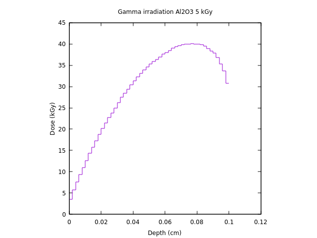
Also could you perhaps explain to me the way the dose is distributed in the attached plot, as I would understand it the dose should be evenly distributed throughout the sample I cannot understand the shape it is exhibiting?
it really depends on your needs. In general the transport threshold should be put at an energy such that the range is smaller than the bin length.
With the file that you shared before I cannot reproduce the above plot. Can you please share the latest *flair file and/or the bnn files that you used to generate the plot?
This is for the exact number of photons I require.
I have removed the source decay and instead just replaced it with a photon beam with the energy of the average of the two photons following the decay process. The only thing I now still am a bit confused about is the bin size and what would be best suited for my simulation. Thank you again for your help.
concerning the bin size, it is something that I cannot tell you, since it really depends on your needs. Once you have decided on the desired resolution, adapt the transport thresholds with the “recipe” above that can be found in the lectures and manual.
Concerning the dose profile, be also very careful since the energy deposition is due to the secondary electrons generated by the photons (photoelectric, compton, pair production): the electron fluence in your target will not be uniform.
The curve that you get for monoenergetic photons is reasonable. My previous query arose because if one simulates an unshielded Co-60 source, the energy deposition in the first layers of the target is much higher due to the electrons from the beta decay that are stopped at the surface. Again, deciding what to use as source depends on your problem and what you need to achieve in the end.
Thank you for your response I added the transport thresholds I thought necessary. The reason I decided to go with the mono-energetic photons is because this lead me closer to what I believe the results to be. However, for accuracy’s sake I think using a 60Co source is better. I am confused now however in what to do post processing as when using a beam I understand the NORM field in the plotting section to enable me to add the number of particles I want but I am unsure how this relates using a decay source.
For example the number of photons interacting with my sample is mentioned above but when I use this for my decay source the plot is very unreasonable. I have done irradiations at cc60 and was told that for this number of photons the delivered dose should be around 5kGy.
If you could have a look at my input file and help me understand why this value is so far off I would really appreciate it.
thanks for your feedback.
If you run a simulation with a radioactive source and RADDECAY in Semi-Analogue mode, the results are expressed per decay. So if you score DOSE, the default output unit will be GeV/g/decay.
You should multiply y the conversion factor to get Gy/decay (as you have already done) and then by the activity of your radioactive source in Bq (i.e. decays/s) and by the duration of your irradiation. This will give you a dose in Gy.
I have made quite a few changes to make my simulation better represent the true irradiation trial my samples underwent. I have created a Co60 source which I believe to be located at the origin. I have moved my sample which is a 1cm diameter disk with a thickness of 0.1cm (Al2O3) and have placed it 80 cm away from the source.
I believe what I have done is more on the right track however I am getting some strange results when analyzing the dose at the region of my sample. Would you mind giving me some insight into where I may be mistaken.
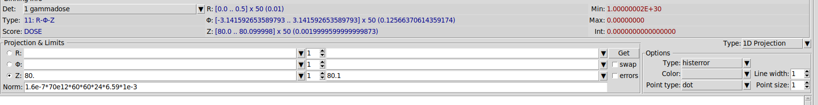
I have uploaded my window from post processing as well as the new files. The source is 70 TBq and should emit photons over a solid angle of 4pi. I have added the 1e-3 at the end of the norm field to convert my results from Gy to kGy.
I don’t know the exact details of your irradiation setup but I can comment on the BEAMPOS card that you added to define a spatially extended source. You are currently defining a spherical source with 81 cm radius (I guess you wanted to include the sample) but most likely this is not the case.
If you have a look at the manual or the lectures, with a spatially extended source the source particles (the decaying isotopes in your case) are sampled within the volume: it is as if you have a radioactive source of 81 cm. I am confident that in reality your sealed radioactive source would be in a rather small spherical or cylindrical volume of the order of ~1cm3 or less. The fluence spatial distribution is drastically different as in the first case your sample sees a distributed source (partially within the sample itself) while in the second case essentially a point source at 80 cm distance. To convince yourself you can score the PHOTON fluence distribution as well
Thank for your effort I really do appreciate it. I understand what you are saying I have changed my BEAMPOS to be a source with a radius of ~ 1cm. What I wish to do is to simply extend the direction of the photons produced by this source in all directions isotropically and to then simulate only the small portion of photons and resulting secondaries my sample receives. I have looked in the online lectures and I find them a bit hard to follow how do I enable my source to do as I wish?
Following this when scoring using the USRBIN I am only sampling from the region of 80cm to 80.1cm as this is the region in which my sample is occupied (the rest is irrelevant).
Any insight you could provide me with will really be appreciated.
The source settings that you have now, are doing what you wish. With ISOTOPE + spatially extended source, the isotope location is sampled randomly in the cylindrical volume you have specified and the direction of the decay radiation is also sampled randomly: the effect is then to have an isotropic emission.
As general suggestion, sometimes it is good to add additional scorers other than the ones one is interested in, especially if they are not a large overhead to the simulation. This can help a lot in better understanding the problem at hand