Electron backscattering in thin foils

[Lovepreet (Lovepreet Singh)]

Versions

Please provide the used software versions.

FLUKA: 4-5.1
Flair: 3.4-5.4

Description

Dear FLUKA experts,

I am comparing 500 keV electron elastic backscattering from an ultrathin tungsten foil between FLUKA and Geant4.

In FLUKA I use PRECISIO and force electron/positron Coulomb single scattering with:

MULSOPT 0.0 0.0 0.0 1.0 1.0 1001.0 GLOBEMF

In Geant4 11.4 I use G4EmStandardPhysicsSS.

I extracted the primary-electron cross section integrated over θ>90 using 0.5, 1, and 2 nm tungsten foils and the results (based on 1e8 primaries) are thickness-independent:

Thickness Geant4 [cm2/atom] FLUKA [cm2/atom] G4/FLUKA
0.5 nm 8.04e-22 5.92e-22 1.36 ± 0.13
1.0 nm 8.45e-22 6.37e-22 1.33 ± 0.09
2.0 nm 8.49e-22 6.24e-22 1.36 ± 0.06

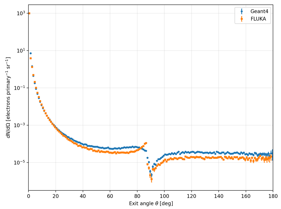
The difference appears largest in the 90–110° angular range and becomes smaller at larger backward angles as can be observed below:

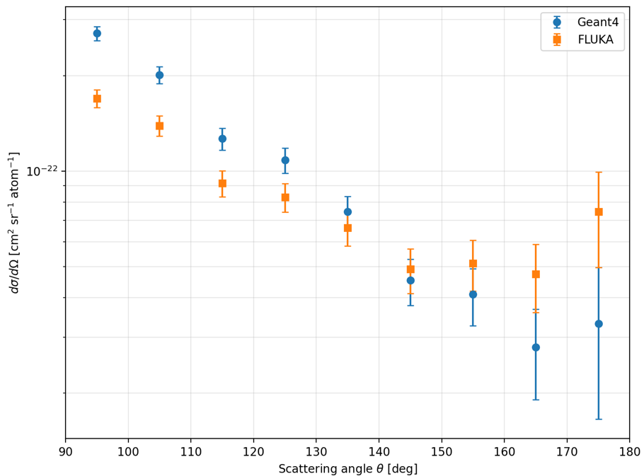
I am trying to understand the origin of this discrepancy between FLUKA and Geant4. Could you please help me determine which differences in the electron elastic-scattering models or transport settings might explain it?

I have also attached the input files for FLUKA.

Thanks,

Lovepreet

thin_foil.inp (1.2 KB)

mgdraw_cross_section_actual_faces_v4.f (3.8 KB)

Input files

Please upload all relevant files. (FLUKA input file, Flair project file, user routines, and data files)

[cesc (Francesc Salvat Pujol)]

Dear Lovepreet,

I understand you’re using the same geometry + scoring for both cases. From your provided input one gathers

i.e. indeed a quite thin geometry along z (2 nm and down to 0.5 nm as per your summary table), but it extends 0.4 cm along both x and y. With the exception of very forward or very backward directions with respect to the beam, electrons will likely undergo several collisions on their way out. Your scoring does not seem to be aware of e- that may have undergone more than 1 collision. It’s not clear to me that the quantity you eventually produce is a differential cross section at all.

I see you’re using the BXDRAW entry in mgdraw.f to intercept electrons from the foil to the void, then dumping electron energy + direction to a file. Then you must have your postprocessing that produces histograms, divides by the subtended solid angle, by the number of primaries, and scales by some (which?) integrated cross section for Coulomb scattering. This is excessive: you can make your life easier (with zero coding) by way of the built-inUSRYIELDcard (you can score angular current with respect to the beam direction as electrons exit from foil to void). If you then restrict the X and Y extent of your geometry to something nanometric, you should get substantially closer to an angular distribution per interaction which you can then scale up to a differential cross section. More on this later if needed.

Going now to the underlying physics substance, could you take your first MULSOPT card

promote it to

and see the effect?

The rationale behind the suggestion: 500 keV for e- is already quite relativistic. The underlying screened relativistic Rutherford differential cross section that FLUKA assumes as a baseline for elastic scattering needs to be promoted to the Mott cross section (Coulomb scattering à la Dirac), which in FLUKA is accessible up to a 2nd-order Born approximation via the suggested card. This typically has an effect in the differential cross section at intermediate and large scattering angles.

This is most exhilarating. Do keep us posted.

Cheers,

Cesc

PS: in all of the above you have delta-ray production activated (threshold at 1 keV as per your input). So some of the e- you intercept are secondaries from ionization events, not from elastic scattering on W atoms. This is perfectly physical - but they smear what you score thinking of just elastic scattering on W atoms. While physical, for your particular purposes you may want to remove them (raise the delta-ray production threshold).

PS2: alternatively, you can be content with an angular current a cross a thin slab and get rid of all scalings etc.

[Lovepreet (Lovepreet Singh)]

Dear Cesc,

Thank you for your comments. I implemented them in steps to observe the differences:

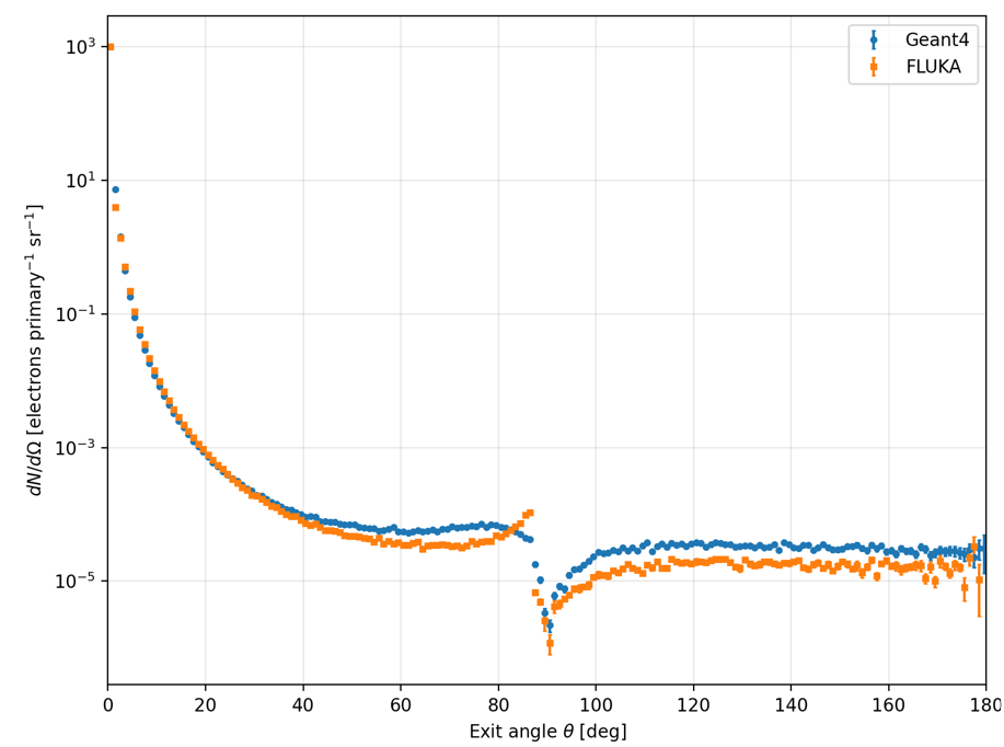
1. Replacing USERDUMP WITH USRYIELD (the rest the same as before). Plotting the angular current across the thin slab I get
   

The difference between the two codes starts to appear above 40 degrees. I also computed the values of the forward and backward integrated currents per launched primary:

===== ALL ELECTRON FOIL → VOID ANGULAR CURRENT =====

Geant4 launched primaries = 100000000

Integrated forward current, theta < 90 deg:

Geant4 = 1.0002433100e+00

FLUKA = 1.0001725979e+00

G4/FLUKA = 1.00007070

Integrated backward current, theta >= 90 deg:

Geant4 = 1.8239000000e-04

FLUKA = 9.7899999998e-05

G4/FLUKA = 1.86302349

Integrated total current:

Geant4 = 1.0004257000e+00

FLUKA = 1.0002704979e+00

G4/FLUKA = 1.00015516

The major difference appears in the backward current

2. Applying the correction in MULSOPT (input file attached)

   

There is a slight increase in the ratio

Integrated backward current, theta >= 90 deg:
Geant4 = 1.8239000000e-04
FLUKA = 9.6869999979e-05
G4/FLUKA = 1.88283266

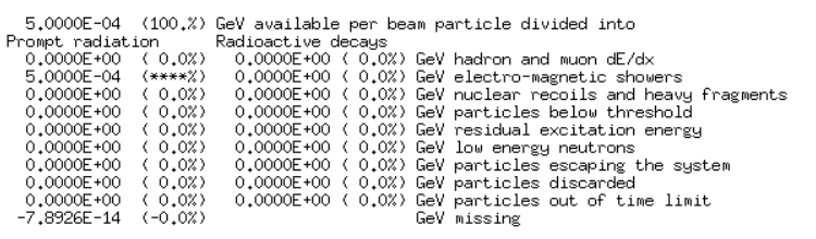
3. If I try to increase the threshold for delta ray production to 0.5 MeV, I get all the primaries depositing their energy in the slab

4. I didn’t change the slab dimensions for now. I would first wait for your comments.

Regards,

Lovepreet

thin_foil_mulsopt.inp (1.4 KB)

[cesc (Francesc Salvat Pujol)]

Dear Lovepreet,

The plot thickens!

1. On theUSERDUMP → USRYIELD upgrade: nice, you spared yourself considerable effort.
2. Requesting spin-relativistic corrections to 2nd order Born approximation you thus far see an increase at intermediate scattering angles (say from 10 to 60 deg). At larger angles you see no effect yet. At 90 deg there’s a geometry/tracking effect due to the de-facto infinite lateral extent of the slab.
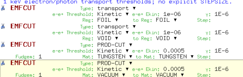
3. On the EMFCUT with PROD-CUT: 500 keV was slightly excessive. Transport cuts (1 keV) are overridden to that value (the code thinks: why to transport e- at energies where you cannot produce), which happens to be at the primary energy, so e- are dumped on the spot.

In order to disentangle things I’d suggest:

• Change the geometry to a sphere of say 1 nm radius (this way we’re not influenced by the artifact at 90 deg and you substantially come closer to an individual-interaction level).
• Put a delta-ray production cut (EMF-CUT) of a few 100 keV instead. Actually, even 499 keV might do. This way we get rid of essentially all secondary electrons.
• Run again with and without spin-relativistic corrections and let’s see.

Once this scenario is clear (you should essentially see Coulomb scattering at an almost individual-interaction level) you can bring back the slab geometry and then the secondary electrons (gradually lowering the delta-ray production threshold), in this way disentangling where differences come from.

Cheers,

Cesc

[Lovepreet (Lovepreet Singh)]

Thanks for your comments, Cesc!

The plot thickens, indeed! In this post, I will show my simulations results while in the next one the comparison with theory.

So, now I have a sphere with prod-cut 499 keV with and without correction (inputs attached).

If I have no correction, the difference is lower:
===== ALL ELECTRON FOIL → VOID ANGULAR CURRENT =====
Geant4 launched primaries = 100000000

Integrated forward current, theta < 90 deg:
Geant4 = 9.9998831000e-01
FLUKA = 9.9997733714e-01
G4/FLUKA = 1.00001097

Integrated backward current, theta >= 90 deg:
Geant4 = 1.1690000000e-05
FLUKA = 8.1099999585e-06
G4/FLUKA = 1.44143034

Integrated total current:
Geant4 = 1.0000000000e+00
FLUKA = 9.9998544714e-01
G4/FLUKA = 1.00001455

Instead with the correction:
===== ALL ELECTRON FOIL → VOID ANGULAR CURRENT =====
Geant4 launched primaries = 100000000

Integrated forward current, theta < 90 deg:
Geant4 = 9.9998831000e-01
FLUKA = 9.9997754511e-01
G4/FLUKA = 1.00001077

Integrated backward current, theta >= 90 deg:
Geant4 = 1.1690000000e-05
FLUKA = 5.5999999543e-06
G4/FLUKA = 2.08750002

Integrated total current:
Geant4 = 1.0000000000e+00
FLUKA = 9.9998314511e-01
G4/FLUKA = 1.00001686

Apart from this, with a prod-cut threshold some electrons are getting killed in the material (the total current is not 1 like in Geant4). I imagine this is due to the threshold.

I tried a threshold of 200 keV as well, but still a factor of 2 with the correction remains:
===== ALL ELECTRON FOIL → VOID ANGULAR CURRENT =====
Geant4 launched primaries = 100000000

Integrated forward current, theta < 90 deg:
Geant4 = 9.9998831000e-01
FLUKA = 9.9999472391e-01
G4/FLUKA = 0.99999359

Integrated backward current, theta >= 90 deg:
Geant4 = 1.1690000000e-05
FLUKA = 5.7699999725e-06
G4/FLUKA = 2.02599654

Integrated total current:
Geant4 = 1.0000000000e+00
FLUKA = 1.0000004939e+00
G4/FLUKA = 0.99999951

thin_foil_w_corr.inp (1.4 KB)

thin_foil_wo_corr.inp (1.4 KB)

[Lovepreet (Lovepreet Singh)]

I compared my simulations results with theory. Hopefully, this helps

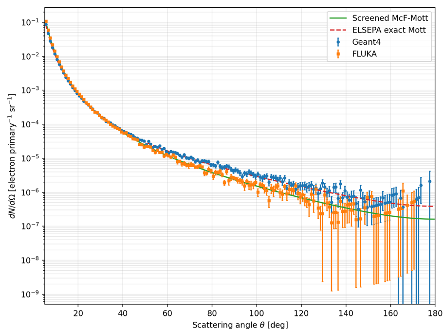
In particular, I compared the two curves from FLUKA and Geant4 with a screened McKinley–Feshbach approximation and an exact Mott calculation with ELSEPA (which solves the relativistic Dirac scattering problem using a partial-wave expansion).

I found interesting results (at least, for me)

Here, I am showing the two curves that I showed above with the 2nd order Bohr correction in FLUKA. The FLUKA curve agrees with McF-Mott curve while the Geant4 curve agrees with ELSEPA exact Mott:

===== BACKWARD CURRENT VS TWO MOTT THEORIES =====
Sphere radius [nm] = 1
Areal density = 1.26443991e+16 atoms/cm^2

Geant4 = 1.1690000000e-05
FLUKA = 5.7699999725e-06
Screened McF-Mott = 5.4242372493e-06
ELSEPA exact Mott = 1.0894813008e-05

G4/McF-Mott = 2.15514172
FLUKA/McF-Mott = 1.06374403
G4/ELSEPA = 1.07298767
FLUKA/ELSEPA = 0.52960982

So, McF-Mott seems to agree with FLUKA while Geant4 agrees with ELSEPA.

Just to be sure, I also compared the two curves without 2nd order Bohr correction with theory. Here, I am showing only the numbers, since the figure is not important:
===== BACKWARD CURRENT VS TWO MOTT THEORIES =====
Sphere radius [nm] = 1
Areal density = 1.26443991e+16 atoms/cm^2

Geant4 = 1.1690000000e-05
FLUKA = 7.9999999204e-06
Screened McF-Mott = 5.4242372493e-06
ELSEPA exact Mott = 1.0894813008e-05

G4/McF-Mott = 2.15514172
FLUKA/McF-Mott = 1.47486173
G4/ELSEPA = 1.07298767
FLUKA/ELSEPA = 0.73429438

So, without the correction, the agreement with the McKinley–Feshbach Mott approximation becomes worse, as expected.

Please let me know if this makes sense to you.

Thanks,

Lovepreet

[cesc (Francesc Salvat Pujol)]

Dear Lovepreet,

Indeed, now that we’ve focused on elastic e- scattering off screened atomic potentials (without interference from geometry or from secondary-electron production) some clarity is attained.

What one sees is the effect of having a full Mott calculation (exact solution of Coulomb scattering with the Dirac equation for a point charge nucleus with infinite mass) vs a 2nd order Born approximation (à la McKinley-Feshbach, indeed), as per the rationale of my first reply.

Nonetheless, one should still consider that, in reality, secondary electrons considerably reshapes the large-angle picture.

To close in even higher spirits, you might be pleased to know that in view of the next generation of the code (FLUKA v5, presently in the making), charged-particle transport will be overhauled. This includes elastic scattering of e-/e+ and heavier charged particles on atoms, as well as ionisation, as a result of an ongoing PhD thesis fully devoted to these topics. Do stay tuned!

With kind regards,

Cesc

[Lovepreet (Lovepreet Singh)]

Dear Cesc,

That’s great. Looking forward to FLUKA v5.

It should be safe to say that even if secondary electrons change the picture, some effects of different cross sections would still survive.

Best regards,

Lovepreet