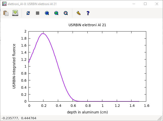
I’d like to simulate the transmission of 3.08 MeV electrons through aluminum of certain thicknesses. I have assumed (wrongly?) that I could obtain it by simulating the depth-fluence curve of a pencil beam impinging on a thick bulk of aluminum and detecting it with a wide enough USRBIN detector (with Part: ELECTRON), able to collect all (or almost all) the electrons. My assumption: the USRBIN-collected value at any depth in the aluminum bulk should represent the relative transmission value one has if at that depth there was an aluminum/vaccum interface.
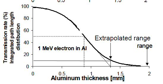
Said that, I get a curve like in the first figure (it looks like a depth-dose curve), however I was expecting to get a buildup-free curve like the one in the second figure (taken from Extrapolated Range Expression for Electrons Down to ~10 eV - Archive ouverte HAL). Can you please help me understand what I’m assuming and/or doing wrong? Thank you in advance.
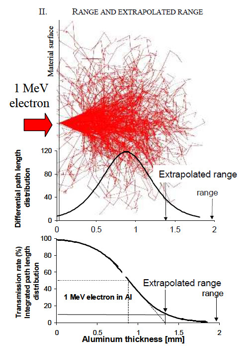
I understand that the bottom curve is obtained as a reversed integral from the top curve:
100% of the electrons enter the target;
~50% of the electrons reach 0.9 mm;
no electrons arrive at 2 mm.
This is not what you’re plotting with Fluka, which is instead a track length estimate and is similar to the top curve from the paper. It’s true that the Fluka curve (I obtain the same as you) doesn’t look like exactly as the one from the paper, but I have to say that the paper doesn’t provide enough details on how the top curve was obtained; I suspect that it is just a demonstrative one.
Instead, I’m able to replicate the top part of the picture. To do that I defined a Cartesian mesh USRBIN with a very fine binning. You cannot obtain it with the USRBIN present in your input as it is a very coarse cylindrical one.
thank you very much for taking the time to check my problem and kindly reply. No problem if my curve does not look like as the top one in the paper, they are different energies and that was not my main purpose. Moreover, I posted the figure of that paper just to show with an example what I was talking about. My actual purpose is to simulate the transmission curve with FLUKA, i.e. the percent of transmitted electrons vs. aluminum thickness. I get from your comment that it is not equivalent to a depth-fluence curve. Can you please elaborate what you mean by “a reversed integral from the top curve”? Do you mean a cumulative integral calculated from say 2 mm backwards to zero? I admit I find it difficult to understand why the fluence integrated over the transversal plane does not reproduce the transmission.
Sorry, I wasn’t clear, I mean precisely a cumulative integral from 2 mm backward to 0 mm.
I wouldn’t expect the fluence (integrated over the transversal plane) to look like as the transmission. Secondary electrons indeed contribute to the fluence and this is why you have an initial increase in the fluence, while the electromagnetic shower is generated, followed by a decrease, when the shower is being absorbed.
Instead, the transmission regards the primaries, it’s about how many primaries can reach a given thickness and this can only decrease, you start from 100% and will end with 0%.
thank you for your further reply. What you say about the secondary electrons is very interesting. Indeed the applicative purpose of my simulation is to compare it with a measurement made by a colleague of the transmission of a linac beam through a few slabs of aluminum, with thickness values 1, 2, 3, 4, 5, 5.5 and 6 mm. The 3.08 MeV I used comes from an elaboration of that measurement. I should assume that only the primary electrons are being captured in her setup because in the experimental depth-current curve she obtains there is no buildup - shouldn’t I?
Regarding the backwards cumulative integral of the transversally-integrated fluence, if I understand it correctly its dimensions are those of a length, while transmission should be a dimensionless quantity. Am I missing something very basic?
I’m sorry, I cannot comment about an experiment I know nothing about.
Instead, why do you say that the dimension of the cumulative are those of a length? You’re integrating over a length a quantity which is #particles per bin-length.
thank you for your patience. You’re right about the experiment, I need to ask my colleague next week. Regarding the dimension of the cumulative integral, here is my reasoning.
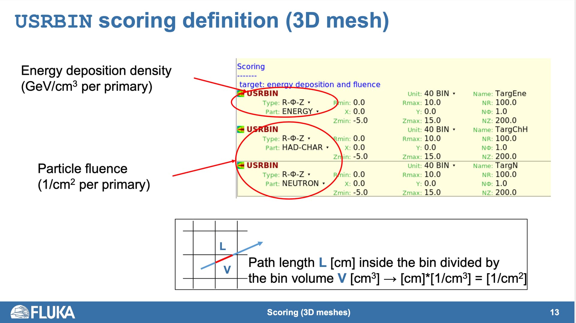
According to the below-shown slide about scoring (from 08_Scoring_I_2021_online.pdf), the “fluence” scored by FLUKA has the dimensions of 1/cm^2 per primary (due to being the volume density of path length). Thus, in my case, it is 1/cm^2 per electron. By multiplying it by the area of the transversal plane, the resulting dimension is 1/cm^2 times cm^2, therefore I obtain a dimensionless quantity (which is the one plotted in the first figure of my first post above). If I further compute its integral over the depth (the “cumulative integral”), I obtain a quantity whose dimension is a length.
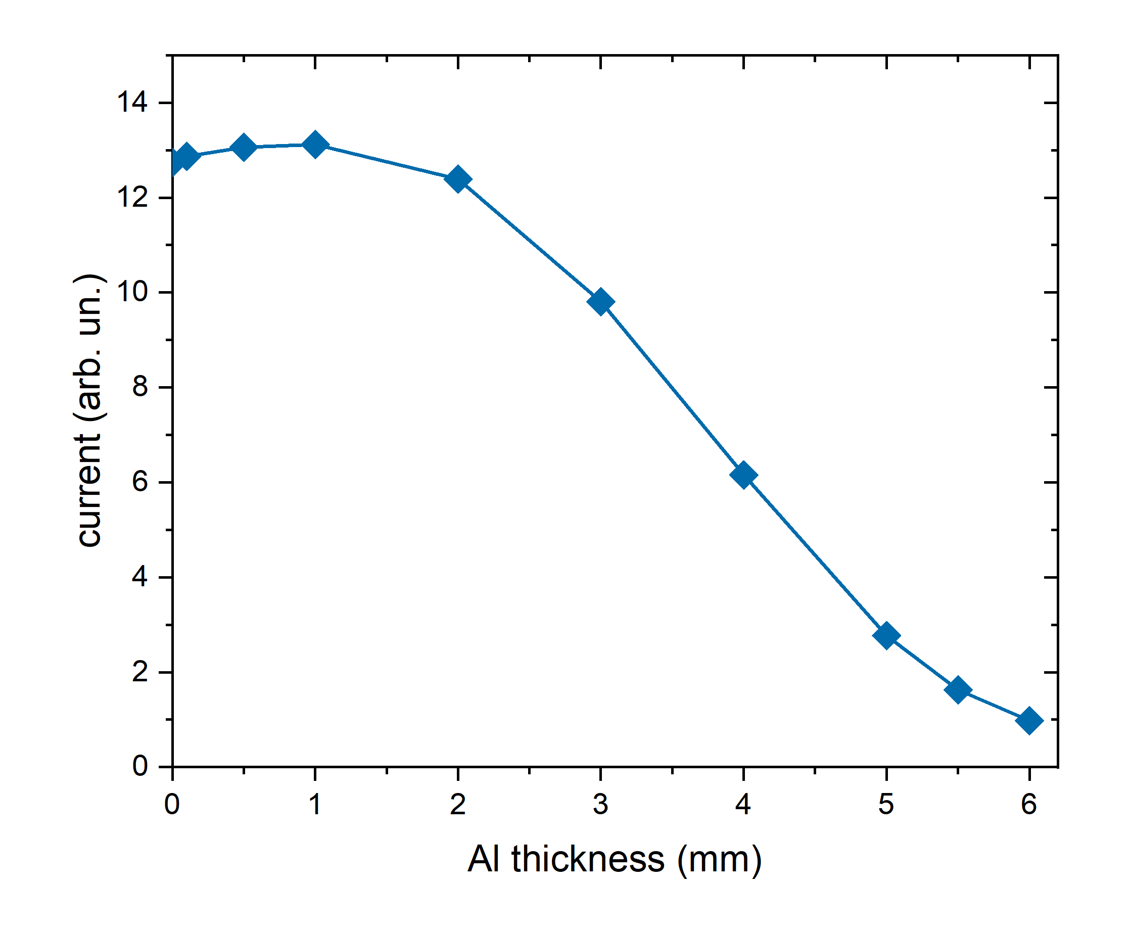
I believe I’ve found out what I was doing wrong. To obtain the transmission, one should estimate the current rather than the fluence. By doing so for the present case, by energy-integrating the current-vs.-energy distributions estimated with USRBDX for a few sampled Al thicknesses, I obtain the following plot, whose shape is now compatible with the literature.