Looking back
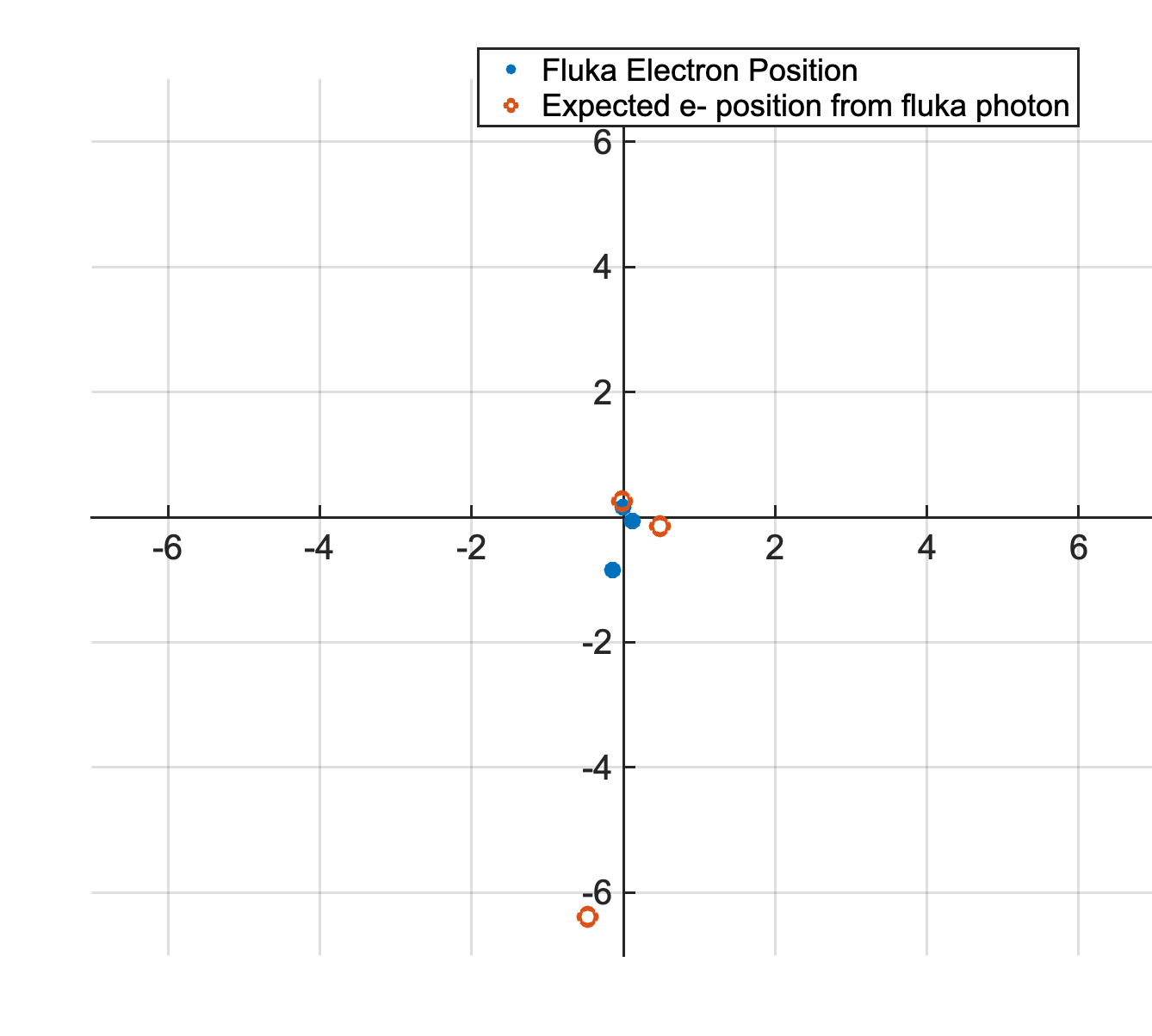
…then you compare your predicted electron position with what you get from the electron-scoring file, implicitly expecting that they should correlate.
Your approach is undermined/flawed by the fact that on its way out of the target, the electron produced in a Compton interaction still undergoes Coulomb scattering, gradually changing its direction. Thus, the electron direction (or position) you intercept at scoring level is no longer the original electron direction from the original Compton interaction - so you should not expect that these correlate. Instead, the e- direction at the exit of the slab is convoluted/smeared by the effect of several deflections on the electrostatic potential of the screened target atoms that the Compton e- encounters on its way out of the (even if thin) layer.
Another major aspect that eluded me on Friday:
I am trying to simulate compton scattering of ~0.004 GeV photons
Lovely. But why does your BEAM card have an energy of 400 keV? You’ll then be in an energy domain where photoelectric effect will still happen at a certain rate (still not dominating but certainly more frequent that at the intended 4 MeV). This leads to an additional flaw in the approach: the electrons you score are not exclusively from Compton interactions!
If you increase the incoming photon energy to 4 MeV, pair production may start to dominate, so a considerable fraction of e- you intercept at your boundary crossing will be from pair production rather than from Compton interactions…
As further higher-order effects (impacting possibly less than 1% of interacting primary photon histories but still noteworthy as possible pitfalls), to name but a few:
- the photons you score are not necessarily the Compton photons. Once in a while there will be Bremsstrahlung photons. Or Rayleigh interactions which deflect the photon direction.
- depending on how you set the delta ray production thresholds, you may even intercept secondary electrons knocked out as delta rays by the Compton electron (or an electron from an occasional photoelectric effect event) on its way out.
Moving forward
You should instead intercept the Compton electron and photon directions at the individual interaction level, by way of the USDRAW entry in mgdraw.f. With this you are sure you intercept the actual events you care about and that you are free from inadvertently flawed assumptions, further interactions convoluting/smearing the information you want, etc.
I did not attempt to derive your expressions. Triple check they’re alright (i was a bit surprised by the lack of the ratio of outgoing and incoming photon energies that appears all the time when one does Compton scattering kinematics, but maybe they’re alright).
For good measure, I made sure the kinematics checks out at interaction level. Let \textbf{p}_\gamma, \textbf{p}'_\gamma, and \textbf{p}'_e be the incoming photon, Compton photon, and Compton electron linear momentum, respectively. Assuming that the target electron is free (unbound) and at rest, a trivial request of momentum conservation,
\textbf{p}'_e= \textbf{p}_\gamma -\textbf{p}'_\gamma
leads (taking the dot product left and right with \textbf{p}_\gamma and applying minimal manipulation) to
\cos\theta'_e
=
\frac
{E_\gamma-E'_\gamma\cos\theta'_\gamma}
{\sqrt{E_\gamma^2+(E'_\gamma)^2-2E_\gamma E'_\gamma \cos\theta'_\gamma}},
or, dividing numerator and denominator in the right-hand side by E_\gamma,
\cos\theta'_e
=
\frac
{1-\tau\cos\theta'_\gamma}
{\sqrt{1+\tau^2-2\tau \cos\theta'_\gamma}},
\qquad
\tau=\frac{E'_\gamma}{E_\gamma}
thus relating \theta'_\gamma and \theta'_e, i.e. the polar angle (with respect to the incoming photon direction) of the Compton photon and electron, respectively, employing a common notation in terms of \tau. NB: E_\gamma and E'_\gamma are the initial and Compton photon energies, respectively.
Here goes an mgdraw.f that intercepts Compton events and writes out Compton photon and Compton electron angles (and a cross check with the kinematics check above). Triple check and adapt it as needed, it’s up to you:
mgdraw.f (11.6 KB)
You’ll notice:
- I am not even assuming that the incoming photon goes along z (just in case there’s a prior photon interaction, unlikely as it may be in a thin layer, but see below…)
- It measures \theta'_\gamma from the final state of the Compton interaction
- It measures \theta'_e from the final state of the Compton interaction
- It evaluates \theta'_e as per the naive expression above (assuming the target e- is free and at rest).
- It writes everything out to unit
70, including the generation of the interacting photon (LTRACK).
- In addition, it writes out to unit
80 a log of all interactions that are not Compton interactions.
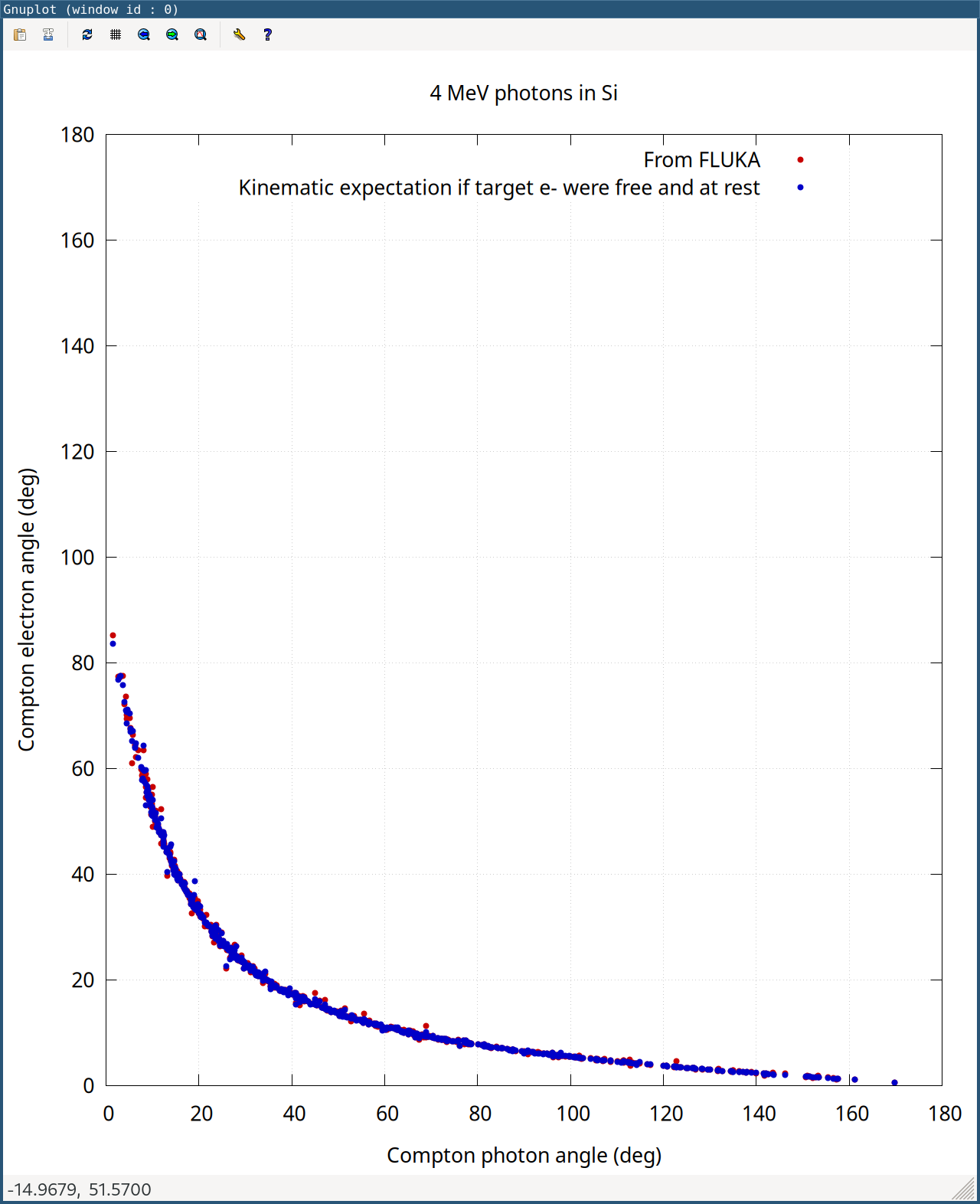
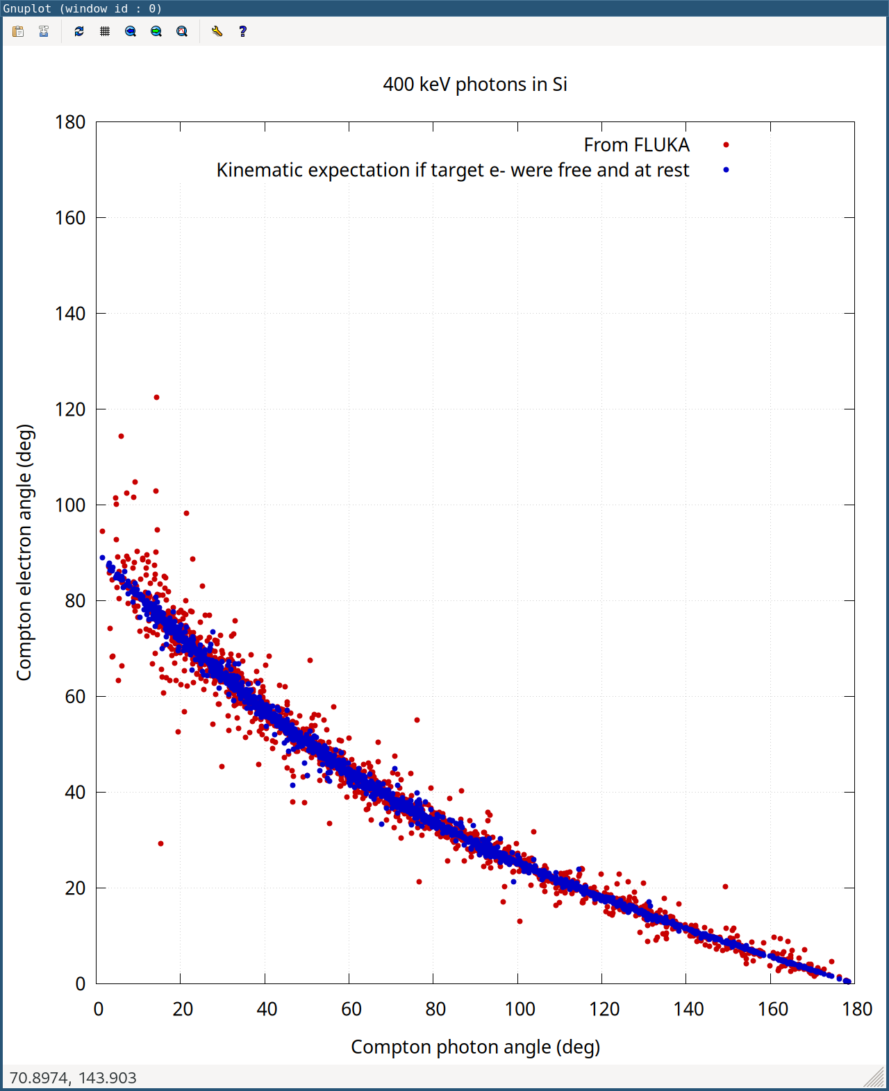
Here goes a plot of \theta'_e as a function of \theta'_\gamma, exctracting the former from FLUKA (red) vs from the simplistic kinematics expectation above (blue) for 4 MeV (actual 4 MeV, not 400 keV!) photons in Si:
Pretty much spot on, except for occasional mild outliers. These are due to the fact that, as opposed to our simple kinematics exercise above where the target e- is assumed free (unbound) and at rest, in reality e- are bound to some atomic shell (so the binding energy should be discounted from the available energy in the kinematics) and they are far from at rest: every atomic orbital \Psi_{n \ell j} has a well defined momentum distribution. FLUKA takes both effects into account.
Certainly at 4 MeV these effects have modest consequences (typical atomic binding energies are in the order of say 10-100 keV), so picturing the target e- free and at rest is a pretty decent Ansatz. If you reduce the energy to, say, 400 keV, the discrepancies with respect to the simple kinematics expectation become more drastic, since at this photon energy one can no longer expect that the simple picture of the target e- being free and at rest is reasonable:
This may also contribute to explain why in your case (inadvertently at 400 keV) you got considerable mismatches, in addition to the points raised at the beginning of this reply.
Finally, just as a curiosity (to stress that photons will not only do Compton scattering in the slab), in the 70 (Compton log) file, you’ll occasionally see Compton-interacting photons with generation number 2 (at least for the 400 keV case). These are then not beam photons (!). I did not run after them, but if i had to take a guess i’d initially think they are Rayleigh scattered or Bremsstrahlung photons. In addition, as expected, in the 80 file (logging all non-Compton interactions) you’ll see a healthy number of pair production events for the 4 MeV primary energy case, and a number of Rayleigh and photoelectric interactions for the 400 keV case.
Hope this helps.
Cesc