Dear Fluka experts,
For a 185 MeV proton beam, I don’t expect there to be Cherenkov radiation in water.
But I do expect for some of the secondary charged particles, such as electrons, to produce the optical photons.
Therefore, I set up a simulation to see if there is any apparent qualitative relationship between the distribution of electrons, by energy, and the spectrum of the resulting Cherenkov radiation.
I have a cylinder of water and some PMMA at the end of it ( trying to simulate a water tank with glass walls). And have tried to only create and transport UV to red light (100 nm to 700 nm).
I have 3 questions:
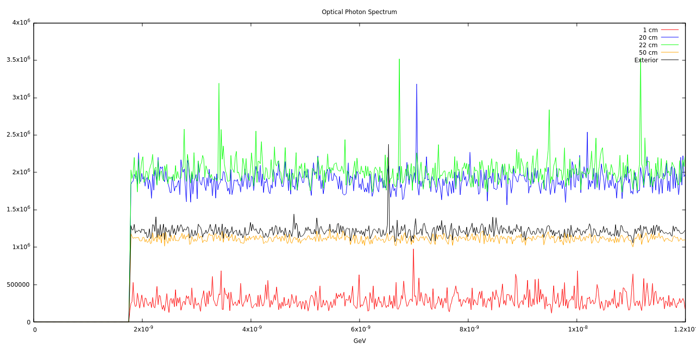
In my “Optical Photon Spectrum” graph, why should I get drop in the count of optical photons when they transport through different materials? Is this an artifact of the parameters of the simulation or physically true? (… guess I don’t know enough optics)
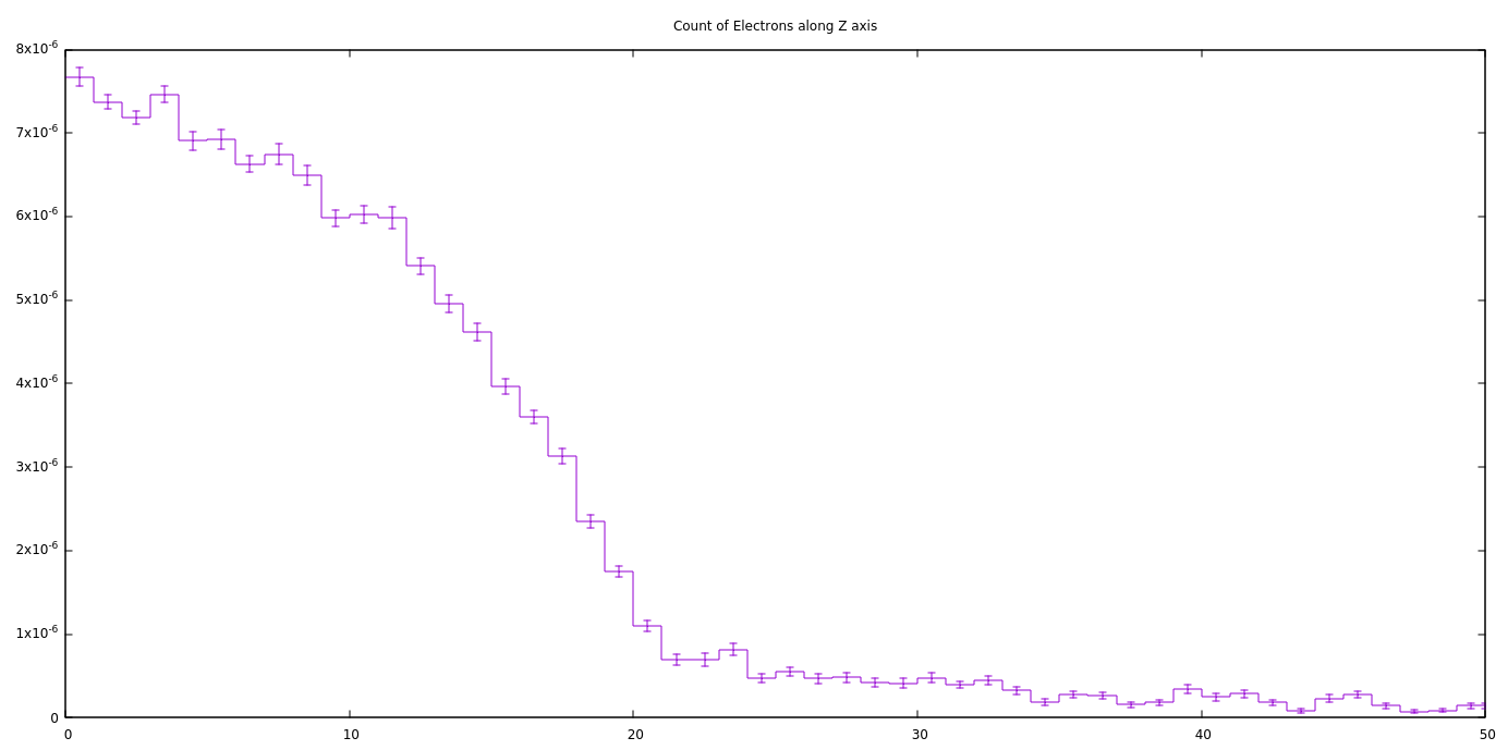
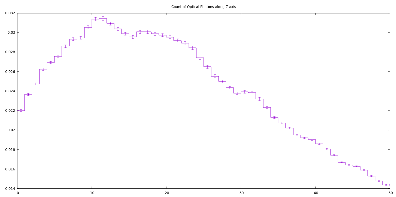
Why are there millions of photons being counted in the same “Optical Photon Spectrum” graph when my “Count of Electrons along Z axis” graph shows few electrons and my “Count of Optical Photons along Z axis” shows a reasonable amount of photons?
Are there other charged particles being transported that accounts for this? ( According to what I have read, I should be getting the rate of photons production by a 0.5 MeV electron at around 10 photons per 0.1 cm.)
Why does my simulation “freeze” when I attempt to add the refractive index for air? (Was playing with this because I wanted to see the spectrum of light a few centimeters away from the tank) Cherenkov_Apr_22_5th.flair (10.1 KB)
For your first question, I suggest you look at the fluence of charged particles in your cylinder of water to get a feel for the density of optical photon creation vertices. I would expect the fluence of photons to overall increase in z since they tend to have their momentum towards the beam direction. Also their number should be very high in the vicinity of the Bragg peak. You should also account for possible absorption in water and escape of photons to air. I cannot provide a straightforward solution because the answer will be unique for each combination of source, geometry and material even with the same optical photon production and transport settings.
For your second question, keep in mind that you are seeing a differential distribution. Therefore, the total number of photons you scored is closer to 0.01 per primary if you integrate. I suggest you look at the simulation summary, at the end of the .out file, which will tells you the total number of optical photons produced.
For your third question, there could be many reasons for that, but I suspect you have optical photons trapped in your cylinder of water because of total internal reflections. When you set the index of refraction for air, the optical photons are either reflected or transmitted at the interface instead of being absorbed. Make sure the absorption coefficient in water is larger than 0.0 and let me know if you experience the same problem.
Looking at what you said for my second question: if I “integrate” my “Optical Photon Spectrum”, then the result should be a linear (if not close to quadratic) relationship for photon count per unit energy.
If that’s the case, would the correct interpretation be that the spectrum of optic light is linear as function of energy?
Also, according to the FLUKA manual, for USRBIN output, when fluence is scored, it is expressed in “particles/cm^2 per unit primary weight”.
For my “Count of Optical Photons along Z axis” graph, if I ran the simulation for 5,000 protons and the cylinder has radius of 50 cm, to get “number of photons” in the y-axis, what would I have to do?
FLUKA uses a simple model for the spectrum of Cherenkov radiation and which is why you see a flat spectrum. The photon count is not related to the deposited energy but rather to the particle charge and velocity. Most importantly, it depends on the energy (or wavelenght) cutoffs you used in your OPT-PROD card. The number of photons does not directly depends on the stopping power dE/dx unlike scintillation (but of course the stopping power itself depends on the charge and velocity of the particle).
Keep in mind that the fluence is not, in general, equal to the current density as it also depends on the angle of incident on the surface (of the bin). To estimate the number of particle travelling along the y-axis in your cylinder, I suggest you divide it in two regions, top and bottom, made of the cylinder material. Then, you can score the current using a USRBDX detector for optical photons crossing between these two regions. The integral of the distribution provided by USRBDX (which you can also see in the “sum” file after compression) is the number of particles, per primary, crossing between the two regions.
I have done what you suggested for the current!
It works well!
Last question!
According to Jackson’s Classical Electrodynamics, energy loss for fast charged particles at a distance is tied to Cherenkov radiation. Section 13.4
The density effect in energy loss is intimately connected to the coherent response of a medium to the passage of a relativistic particle that causes the emission of Cherenkov radiation.
So, if I wish to add this to my simulation, how would I begin to write the user routine?
Density effects are a reduction in the stopping power compared to the Bethe-Bloch formula explained by the polarization of a dense medium by an incident relativistic particle. That polarization reduces the possible energy transfer from the indicent particle to electrons far away in the medium. When the wavelength of the induced electric field is purely imaginary, which happens in case \beta^2\epsilon(\omega)>1 with \epsilon being the dielectric constant, radiation propagates to infinity as Cerenkov radiation.
The amplitude of the density effect correction can be computed using the Sternheimer’s parameterization. See Eq. 34.7 of Chapter 34 from the PDG for details. You can yourself fine-tune these density effect parameters using the STERNHEIme card. FLUKA already computes which Sternheimer parameters it thinks are the most suitable for the materials you are using. You can see the values which were used in the .out file and see if you are satisfied with them. Otherwise you should use a STERNHEIme card. As it is already handled by FLUKA I see little need for a user routine. Did you have something else in mind?