Source flat distribution in sin^2 (Theta)

tuneu · 13 December 2024 13:32

Dear FLUKA experts,

I am using FLUKA to simulate the development of a cosmic-ray-induced air
shower in the Earth’s atmosphere and track the muon propagation several
meters underground. My simulation layout consists of a cylindrical
detector employing a 100th multilayered atmosphere up to about 70 km
above sea level, adding a few layers below the ground level. For the
cosmic ray injection, I am currently using the annular distribution
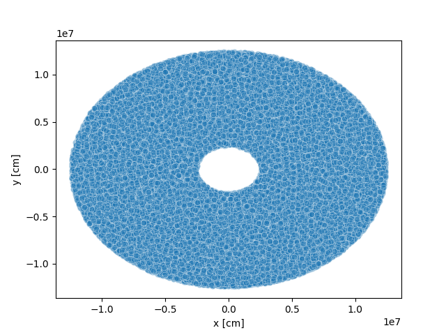
available in the source new gen file (5.2.3). My results are shown in
the attached figures. The first shows the annular distribution XY plane at the top of te atmosphere, and the second te sin^2 \theta distribution, obtained from the z-component director cosine

annular_XY_plane

sin2Theta_distribution

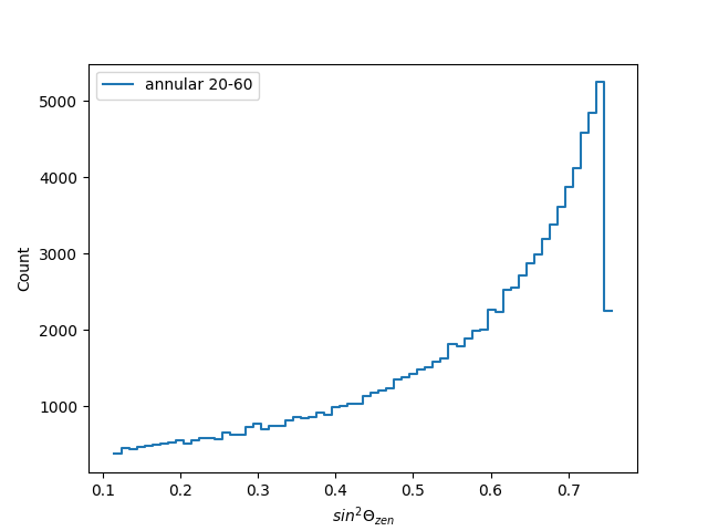
I aim to simulate cosmic rays entering the atmosphere with zenith
angles, theta, comprising 20 - 60 degrees. In such a case, in order to
reproduce the observations as seen by a plane detector, I expect to
inject these cosmic rays according to a flat distribution in sin^2 \theta
from the z-component director cosine. However, from my figure, using the
annular distribution, the injection points of cosmic rays seem to be
uniformly distributed over the whole area defined between r_min and
r_max. This distribution generates an excess of extensive air showers at
higher zenith angles when I would want the opposite. Is that the case?
In this sense, I would like to ask you if you have available a FLUKA
subroutine that generates a flat distribution in sin^2 theta.

I have attached a simplified input, usrdraw, and source_newgen to reproduce those results.
Also, a short code in Python to read the output since I am not using any Fluka Plot tool in this input.

annular_20_60.inp (2.7 KB)
usrdraw_fluka_forum.f (7.4 KB)
read_primaries_annular.py (678 Bytes)
source_newgen_anular_20_60.f (20.6 KB)

Many thanks!

All the best,

gmazzola · 17 December 2024 10:28

Dear Jordi,

thanks for your question!
Allow me some time to have look and understand how to best approach your inquiry, I will answer you as soon as I can.

Cheers,
Giuseppe

tuneu · 17 December 2024 15:23

Dear Giuseppe,

Many Thanks for your time.
I’m still working on some tests to implement it in FLUKA. Let me share what I’ve reached so you can better guide me.

Into an external code I generate 10000 uniform points between sin^2 \theta_{min} = 0.113872 to sin^2 \theta_{max} = 0.756727 (angle range of interest ) and I computed the radial distances:

r = h \times \sqrt{\frac{sin^2 \theta}{1 - sin^2 \theta}} ,
where h is the altitude (72 km)

Finally, I rewrite r in Cartesian coordinates x and y. The next figure shows the annular distribution from FLUKA (orange) and the annular distribution producing a uniform distribution in sin^2 \theta (blue). Note that, even though there are fewer blue points, the limits of both annular distributions agree (better seen in the cos_z \theta distribution)

I am trying to export this distribution in FLUKA, and based on the sample_annular_distribution from FLUKA, I have implemented this piece of code in the source_library.inc (I’m unsure if including a new source in the source_library.inc is the best way to proceed instead of doing it directly in the source_newgen file.):

subroutine sample_annular_distribution_sin2theta( rmin, rmax, axis_1, axis_2)

     use source_library

     implicit none

     double precision rmin, rmax, axis_1, axis_2
     double precision sin_theta, cos_theta, sin2_theta_min, sin2_theta_max, sin2_theta
     double precision radius, rmin_squared, rmax_squared
     double precision constant
     double precision FLRNDM, xdummy
     double precision h

     h = 7200000.0D0

     call SFECFE( sin_theta, cos_theta )

     rmin_squared = rmin * rmin
     rmax_squared = rmax * rmax

     constant = TWOTWO / ( rmax_squared - rmin_squared )
     sin2_theta_min = rmin * rmin / (h * h + rmin * rmin)
     sin2_theta_max = rmax * rmax / (h * h + rmax * rmax)
     sin2_theta = TWOTWO * sin2_theta_min + (sin2_theta_max - sin2_theta_min) * FLRNDM ( xdummy )
     
     radius = h * sqrt(sin2_theta /  (1.0 - sin2_theta))
    

     axis_1 = axis_1 + radius * cos_theta
     axis_2 = axis_2 + radius * sin_theta

     return
  end

This code works partially. Using the same r_min, and r_max I’ve used in the annular distribution I’m obtaining different limits for the z-component of the direction cosine distribution.
Below are the plots for XY plane distribution at 72 km, the sin^2\theta distribution (flat as expected), and the component z of the direction cosine from 0.48 to 0.88 I was expecting from 0.5 to 0.94.

When implemented externally the limits are right, so I’m missing something in the FORTRAN code.
I hope that could help.

Many thanks,

Jordi

gmazzola · 21 December 2024 10:09

Dear Jordi,

from a quick look to the python code, it looks like to generate the plots you are showing, you are using the file written in unit 60 by the mgdraw.f routine you attach.

If I then look at the mgdraw.f, the unit 60 file is written in both entry BXDRAW and USDRAW. The first entry writes the information of muons crossing specific boundaries in your geometry (but you are interested in proton, so we can exclude this part). At the second entry, you are writing the information of protons (JTRACK .EQ. 1) but once they undergo an inelastic scattering with secondaries (ICODE .EQ. 101).

My understanding is that you want to check if the primary protons you are loading in your simulation follow the distribution you desire. Therefore, the small difference you see in the cosz might be due to the fact that you are extracting the information of the protons only when they undergo inelastic scattering and not when they are first loaded in the simulation.

I would suggest to use the mgdraw’s entry SODRAW (manual) in order write the information of protons as soon as they are tracked. If the difference is still present afterwards, I will have a deeper look into your simulation.

Cheers,
Giuseppe

tuneu · 2 January 2025 15:30

Dear Giuseppe,

If I then look at the mgdraw.f, the unit 60 file is written in both entries BXDRAW and USDRAW. The first entry writes the information of muons crossing specific boundaries in your geometry (but you are interested in proton, so we can exclude this part). In the second entry, you are writing the information of protons (JTRACK .EQ. 1) but once they undergo an inelastic scattering with secondaries (ICODE .EQ. 101)

Your observations are correct. In the mgdraw.f you have found some code lines in BXDRAW but as you mentioned is irrelevant for this entry. I’m interested in implementing the source function I have mentioned. Also to run faster the example I modified the initial energies. In my simulations, the primary energies are higher, and at the point of inelastic scattering (ICODE .EQ. 101), the cosz doesn’t change too much.

I have followed your suggestions using SODRAW and ignoring the rest (USRBDX and USRDRAW), find attached the USRDRAW file with the modifications.

Unfortunately, I’m not getting the expected results. I was trying to compare the cosz of source functions (sample_annular_distribution vs sample_annular_distribution_sin2theta). For the last the z position is at 72 km, the ltrack is 1 and, the atrack is 0 so it seems that it is pointing at the first particle step. The problem is I’m releasing 100,000 particles and I just get around 16,000 lines. When I use the same input and mgdraw but the original sample_annular_distribution in the source_new_gen.f I get a blank file, so nothing is written.

Is the SODRAW well implemented?

usrdraw_fluka_forum_sodraw.f (6.6 KB)

Many thanks,

tuneu · 6 January 2025 09:04

Dear Giusepe,

I found a bug implementing the subroutine sample_annular_distribution_sin2theta. This code solves the cosz divergences by comparing the original sample_annular_distribution available in the new_source_gen.f

subroutine sample_annular_distribution_sin2theta( rmin, rmax, axis_1, axis_2)

     use source_library

     implicit none

     double precision rmin, rmax, axis_1, axis_2
     double precision sin_theta, cos_theta, sin2_theta_min, sin2_theta_max, sin2_theta
     double precision radius, rmin_squared, rmax_squared
     double precision FLRNDM, xdummy
     double precision h

     h = 7200000.0D0
     call SFECFE( sin_theta, cos_theta )
     rmin_squared = rmin * rmin
     rmax_squared = rmax * rmax

     
     sin2_theta_min = rmin * rmin / (h * h + rmin_squared)
     sin2_theta_max = rmax * rmax / (h * h + rmax_squared)
     sin2_theta = sin2_theta_min + (sin2_theta_max - sin2_theta_min) * FLRNDM ( xdummy )
     radius = h * sqrt(sin2_theta /  (1.0 - sin2_theta))

     axis_1 = axis_1 + radius * cos_theta
     axis_2 = axis_2 + radius * sin_theta

     return
  end

The plots below show the annular distributions, the distribution in sin^2 \theta and cos_z \theta. Now the divergence in cosz has disappeared and the distribution in sin^2 \theta is flat.

The cosz are obtained for the first inelastic interaction using the entry USRDRAW and not from its first appearance as you suggested using SODRAW because I could not write the information correctly. If you can help me with the SODRAW entry I can compare both distributions and close this discussion.

Many thanks and have a happy new year!

Jordi

gmazzola · 6 January 2025 09:41

Dear Jordi,

happy to see that the discrepancies are now being solved!

Regarding the suggestion to use SODRAW entry, in order to directly use the direction of the source particle, the problem in your routine is that you are using the variables contained in the trackr.inc instead the ones from flkstk.inc.
At the level of the SODRAW entry, the source particle is not yet transported, therefore the trackr.inc variables do not contain its information.

In order to obtain the properties of the source particle, I suggest to implement the following lines:

  ENTRY SODRAW

  IF ( .NOT. LFCOPE ) THEN
     LFCOPE = .TRUE.
     IF ( KOMPUT .EQ. 2 ) THEN
        FILNAM2 = '/'//CFDRAW(1:8)//' DUMP A'
     ELSE
        FILNAM2 = 'detections'
     END IF
     OPEN ( UNIT = 60, FILE = FILNAM2, STATUS = 'NEW')
  END IF

  WRITE (60,*) ( 600, ILOFLK(I), LOFLK(I),
 &                    SNGL (TKEFLK(I)), SNGL (PMOFLK(I)),
 &                    SNGL (AGESTK(I)), SNGL (XFLK (I)),
 &                    SNGL (YFLK (I)), SNGL (ZFLK (I)),
 &                    SNGL (TXFLK(I)), SNGL (TYFLK(I)),
 &                    SNGL (TZFLK(I)), I = 1, NPFLKA )     
  RETURN

Happy new year to you too!
Giuseppe

tuneu · 6 January 2025 10:43

Dear Giuseppe,

Thanks for the clarification. The SODRAW entry works as expected now, showing the particle’s first step at the top of the atmosphere. No cosz divergences appeared comparing distributions and the flat distribution in sin^2 \theta works well.

I’ll mark my previous answer as a solution because of the title of this forum entry. It’ll be easier to find how to implement something similar for any interested user.

Many thanks for your help,

All the best,

Jordi