Strange Pattern in USRBIN-DOSE Scoring Result

Dear FLUKA experts,

During my attempt to get the absorbed dose map of a Co-60 source pencil in the air, I got strange DOSE scoring results.

I used BIASING cards to improve statistics by dividing the air into layer regions and assigning the imp-E values in multiples of 2, and there was a strange pattern in the USRBIN-DOSE score as shown below:


There were sawtooth-like distributions at the intersection of the air layer regions.

Then I turned the area into layers of nested cylinders it showed again. It seems that the sawtooth-like distributions are always shown at the edge of the regions. Curiously these strange patterns appear only in the scores for DOSE, which are satisfactory for PHOTON.
Here are the maps of DOSE and PHOTON:


And the input files are here:
v8-std-new-biasing.flair (21.9 KB)
v8-std-new-biasing.inp (5.5 KB)

I suspect the reason for this is the problem of regions division, which leads to less accurate calculations on the boundary, yet there is nothing strange about the statistical results for photons.
It is very confusing and I would like to hear your suggestions.

Best regards,
Shan

Dear @Jungle

Note that this scenario is a good example of when it is not advisable to use region importance biasing. You have a low-density medium, therefore your particles do not interact much with it. This means that the replicas created in the boundaries between regions with different importance will, very likely, have a correlated history, giving rise to potentially poisoned results. Importance biasing is meant to compensate for attenuation by enhancing the amount of particles reaching regions they would reach in very low numbers if no biasing is issued. As you can see, this is not your case, because your photons have no problem crossing the air. Here is a lecture on biasing that may be of help:

Instead, the problem you are facing is that your photons interact little with air and therefore it takes many primaries to obtain your dose results with small statistical uncertainty.

Are you really interested in the dose in the air or maybe in dose equivalent around your source? In the latter case you can select DOSE-EQ in your scoring and the low statistics problem will go away. The DOSE-EQ is calculated using the particle fluences and fluence-to-dose conversion coefficients. Since you have no problem achieving fluence results with low statistical uncertainties with no biasing, the same will apply to DOSE-EQ. Note also that many fluence-to-dose coefficients are available in FLUKA and you can select them using the AUXSCORE card if needed.

Hope this helps and do not hesitate to say so if it does not.

Kind regards,
Francisco

Dear @fogallar ,

Sorry for the late reply. After reading your reply, I remembered some queries that may not have been expressed clear:

  1. the purpose of using BIASING: Since I am using an isotropic Co-60 source, I want to compensate for the primary particles (photons/cm3) that become rare because of the larger radius and space by using BIASING to keep good statistics at a greater distance (e.g. 1m).
  2. whether to try to turn off the BIASING option: I later tried to turn off the BIASING option, but the results obtained were not convergent enough and also still showed similar patterns, so I wonder if this is due to spatial division.
  3. about absorbed dose: Yes, my aim is to get such an absorbed dose field for a Co-60 source at a certain distance. I thought the absorbed dose was calculated in the same way as the dose equivalent, based on the fluence of particles multiplied by some conversion factor. But now I don’t think so.

Besides, the images attached in the last post were obtained by scoring both PHOTON and DOSE in one simulation with BIASING, so I’m very confused.

Best regards,
Shan

Dear @Jungle,

I am taking a look to the pattern issue to fully understand it, and will come back to you asap.

In the meanwhile, you can achieve your map with good statistics and without pattern very easily:

  1. Remove all your biasing (your photons do not become rare at 1 meter distance, not at all).
  2. Remove your many air regions, just keep one big region around your source.
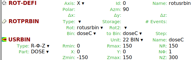
  3. Exploit the cylindrical symmetry of your problem to gain statistics easily → define a cylindrical USRBIN with a reasonable number of bins. You can do for instance as below. Note that you need the ROT-DEFI and ROTPRBIN cards to rotate your USRBIN, since the cylindrical symmetry of your problem is not aligned with the z axis.

image

Hope this helps,
Francisco

EDIT:
You should also reduce your transport and production thresholds for e-/e+/gammas, see the reply below.

Hello again,

Precious information is contained in the FLUKA courses material! :slight_smile:

Your pattern is due to the use of not-optimal transport thresholds for e-/e+/gamma for a USRBIN
with such a fine binning as yours. The transport threshold should be set such as the range of your particles in your material (air) is smaller than the width of your bins. Please check out the lecture below:

You were using the default thresholds of the PRECISIO defaults: 100 keV for e-/e+ and ~33 keV for gammas. The e- range for such energy in air is of the order of 13 cm! And your bins are of the order of 1 cm width.

If you lower your e-/e+ threshold to 10 keV (range ~0.24 cm) and that for gammas to 1 keV, then your pattern should disappear (let me know if it does not). You can do so by means of the EMFCUT card. Do not forget to reduce also the production thresholds to the same level.

My advice is not to go to a finer mesh than necessary and then set your thresholds accordingly. Note that everything said in the previous reply still applies.

Many thanks to H. Vincke and C. Theis for the offline enriching discussion.

Hope this helps,
Francisco

PS: Thresholds are important! See below an example of what one manages to get when messing around with thresholds:

3 Likes

Dear @fogallar ,

Thank you for your patience and detailed discussion. I am trying to use and understand ROT-DEFI and ROTPRBIN options based on your suggestion.

On the other hand, I really didn’t take into account the threshold of e-/e+ or gammas. Your reminder is much needed. Some adjusted simulations are running now. I will let you know when I get satisfactory results.

Thanks again for your help in this matter!

Best regards,
Shan

1 Like

Dear @fogallar

I have tried to lower the thresholds for e-/e+ and gammas. Simulations were performed for two conditions, and 1e7 primaries* 5cycle* 100runs was used for each simulation:

  1. Set e-/e+ threshold to 10keV and for gammas to 1keV

  2. Set e-/e+ threshold to 1keV and for gammas to 1keV

Those patterns that appeared before still reappeared, only they became less obvious.

Besides, when I used AUXSCORE to separate the ELECTRON and PHOTON dose, I found that essentially all the doses were from ELECTRONs.


Is this because the gamma energy is always transformed into the energy of the secondary electrons produced and deposited; while the doses of “PHOTONs” recorded are actually from PHOTONs that are killed below the transport threshold?

Best regards,
Shan

Hi @Jungle,

Please share your updated input file so I can take a look.
In the meanwhile, we already discussed that you do not need importance biasing and that the reason behind the pattern is threshold-related, why keep the subdivision of the air around your source in many regions?

Cheers,
Fran

Dear @fogallar ,

Here are the files:
0709-threshold.inp (6.0 KB)
0709-threshold.flair (41.4 KB)

The use of two sets of threshold settings is to check the effect of thresholds on the results, but the results indicate little difference between 1 and 10 keV on e-/e+. The only obvious difference is in the calculation speed, which is about 2.35ms/prim and 0.33ms/prim respectively.

Besides, previous results show that the pattern appears with or without BIASING option but not for the subdivision of the air, so I added that to obtain good statistics.

Best regards,
Shan

Dear @Jungle,

I see in the input that you have ignored most of the advice given in our previous discussion.
Let me then be more explicit:

The image above results from a simulation that took 76 CPU minutes in my laptop, as opposed to the 1360000 CPU minutes that would take to obtain the results you have reported above using the same number of primaries you have used, also on my laptop. Note the factor ~18000 between both. Those results are obtained by implementing the three points of my initial reply and reducing the threshold, as proposed in my second reply.

So, let me stress once again that the use of importance biasing here is pointless and detrimental. You are splitting photons as they cross regions, effectively simulating more photons, wasting CPU time that would be better employed simply simulating more primary photons, which have completely uncorrelated histories, as opposed to what happens with the ones generated via splitting.

On a secondary note and for completeness (hopefully not diverting your attention from the main point above): the patterns are a consequence of the transport cuts, in combination with your USRBIN and geometry. I ignore the technical details giving rise to them, but I suspect they are related to the influence of boundaries on the transport of electrons approaching them. The consequences of this are very much reduced by lowering the energy cuts, as you have observed. Once this is done, my advice would be to remove the futile region subdivision to avoid any potential impact of such boundaries, which is anyhow my initial advice.

I hope this helps,
Francisco

PS1: I see the dose map in your plots is elliptical, which I believe would be the case if no Co is filling your source region. I assume you have run those simulations without it.

PS2: attention to the FUDGEM parameter when defining the production thresholds!

1 Like

I forgot to mention that separating photon and electron dose is indeed tricky because, as you indicated, the energy is ultimately deposited by electrons and therefore the split between both is affected by the cuts in place.

1 Like

Dear @fogallar ,

I have run the simulation again (1e11 Primaries) with just one air REGION and default thresholds, and obtained similar results to you. The following pictures show the DOSE distribution at Z=100:

In another simulation (without any importance biasing), I also found this phenomenon: the scoring for DOSE and ELECTRON still produced odd, unsmooth patterns at the intersection of some regions. And this reminds me that DOSE is ultimately contributed by electrons, so the root of the previously described ‘pattern’ lies in the distribution of electrons. Here are the results (material in the rectangular areas are also AIR):

So I think we can conclude the following:

  1. The setting of the regions affects the distribution of electrons, which in turn leads to the above pattern of DOSE scoring. (But why does this “imprecise” situation occur in PERCISIO mode?)
  2. The pattern can be improved by lowering the threshold of e-/e+.

Best regards,
Shan

Dear @Jungle,

obtained similar results to you

Great. A couple of notes in passing:

  • It is recommended to reduce the thresholds in accordance to the size of your USRBIN, even if you have only one air region, as we have already discussed and as explained in the already shared lecture.

  • I believe you are using a cartesian USRBIN. Note that using a cylindrical one would significantly reduce the number of primaries needed to achieve results with similar statistics —and the same useful information— than those you show in your reply.


the root of the previously described ‘pattern’ lies in the distribution of electrons

Yes, of course, that is why reducing the electron transport cut had such a clear effect on your results.


Regarding your conclusions:

why does this “imprecise” situation occur in PERCISIO mode?

Please note that PRECISIO defaults does not mean “perfect precision in all cases”. Those defaults are only a compendium of simulation choices, which is detailed in the manual, that provides precise results for most applications. The user can and should tune these choices when appropriate.
There are cases in which one needs a more detailed simulation of the transport of charged particles, and this can be done switching on single scattering, at the cost of higher CPU calculation times (please take a look to the lecture above, in particular the section about Coulomb scattering). But this is not your case, your issue can be solved simply by removing unnecessary boundaries, as you have seen.

The pattern can be improved by lowering the threshold of e-/e+.

Indeed.

Kind regards,
Francisco

Dear @fogallar ,

Thank you for your long term help and detailed explanation on this issue.

I began to understand the importance of setting different transport parameters for different simulation scenarios, especially the EM thresholds.

Thanks again for your help!

Best regards,
Shan

1 Like