Dear experts,
The query is regrading the use of LAM BIAS card. In the present case, 1 GeV proton beam is incident on a copper target of dia = height = 63.744 cm. From fluka .out file, inelastic scattering length of 1 GeV proton in copper target is 14.85 cm.
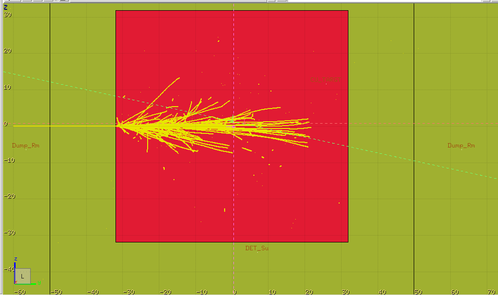
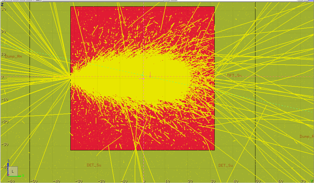
I have carried out two simulations: one without LAM BIAS card and another one with LAM BIAS card setting lambda inelastic = 0.02 for proton in copper material. The corresponding USRDUMP plots (proton beam plot) are attached here. My query in this case is how the physics is conserved here if LAM BIAS is used. From the 2nd figure, it is seen that the proton beams are coming out of the copper target (red portion) whereas from the 1st figure, it is seen that protons are absorbed in the copper target (which is expected in a Dump room).
Hence, using LAM BIAS, the proton flux is different. Due to this, the generated neutron flux may vary. In this context, it will be helpful if you kindly explain how the physics is conserved here ? Or do I have to incorporate any correction in the output if LAM BIAS card is used?
- Without LAM BIAS
- WITH LAM BIAS:
Regards,
Riya