Unexpected normalized dose reduction values of polyethylene shield from DOSE USRBIN

Dear FLUKA experts,

I am using FLUKA/flair to assess the dose reduction of different material (composites). I am a beginner and for that reason start doing simple shield simulations to get acquainted with the software.

One of these simple simulations is to assess the dose reduction of a polyethylene shield with varying thickness and different particle beams at varying energies. Moreover:

  • The thicknesses of the shield are 20 cm and (more extremely) 100 and 200 cm, this is just to see what kind of results are produced
  • The DOSE and DOSEQLET of a water phantom directly behind the beam is used to calculate the dose reduction
  • To calculate the dose reduction, one situation without a shield is simulated as well
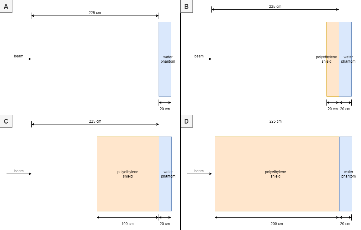
  • The distance between the radiation beam and water phantom for all situations is the same (i.e. 225 cm)

The four different situations are depicted below. Situation A: no shield, Situation B: 20 cm shield, Situation C: 100 cm shield, Situation D: 200 cm.

There are two matters I came across I wanted to discuss.

First, the resulting dose reductions from the DOSE USRBIN were quite unexpected for high energies. At 1 GeV for proton particles the dose reduction is:

  • -21%, 1% and 54% (for 20 cm, 100 cm and 200 cm respectively)

At 10 GeV for proton particles the dose reduction is:

  • -75%, -274% and -282% (for 20 cm, 100 cm and 200 cm respectively)

At 1 GeV for neutron particles the dose reduction is:

  • -75%, -111% and -22% (for 20 cm, 100 cm and 200 cm respectively)

For 10 GeV protons and 1 GeV neutrons, the dose increased for all the thicknesses. I do assume secondary radiation takes part, but not in these large quantities that dose increases over 200% were attained. For this reason, I checked my Input settings to see whether some things were wrong but I did not come across such a thing. Because I’m a beginner, I wanted to ask you if you see anything extraordinary in my input settings. I have attached the inp and flair file herebelow for 10 GeV protons (when I simulate other shield thicknesses, the only changed variable is the Zmin for the RPP shield geometry. In the case of changing the energy and radiation, this is merely changing the ‘E’ and ‘Part’ of the BEAM card). If nothing seems extraordinary, do you maybe have another idea why these huge dose increases resulted?

sim4_1_GCR_pro_10GeV.flair (2.6 KB)
sim4_1_runsA.inp (2.0 KB)

Secondly, when I wanted to assess the DOSEQLET and DOSE for a 1 GeV Helium4 radiation beam in the case of no shield, I get the following error:

Ion beam above BME limit with no rQMD and no or incompatible IONSPLIT option! Execution terminated.

I checked some documentation online (e.g. Re: [fluka-discuss]: Ionsplit and rQMD from Paola Sala on 2020-07-18 (fluka discuss archive)) where it was mentioned that rQMD is used from 130 MeV/n up to 5 GeV/n. While the energy of 1 GeV is within this range, the error message still says there is no rQMD and no or incompatible IONSPLIT option. I am confused about what this exactly means now and why I got the error message. Do you know why this error occurred? I have included the related files herebelow.

sim7_0_GCR_He4_1GeV.flair (2.7 KB)
sim7_0_GCR_He4_1GeV.inp (2.0 KB)
sim7_0_runsA.inp (2.0 KB)
sim7_0_runsA.out (738 Bytes)
sim7_0_runsA001.err (258 Bytes)
sim7_0_runsA001.out (9.5 KB)

I hope I explained everything clearly, if not I can clarify further where necessary.

Many thanks in advance!
Kim

Hi Kim,

the second issue may be simply due to the fact that actually you do not use rQMD as required. To do so, you need to explicitly select, rather than the standard executable that is taken by default, the dedicated executable including the rQMD and DPMJET libraries (bin/flukadpm). In Flair the Exe field of the Run tab allows you to perform this selection.

As for the dose evolution as a function of the shield thickness, which results do you look at? You ask both for a spatial distribution of the dose (then which value do you consider out of it?) and the average over the PHANTOM region (to be still divided by the region volume in cm^3 to actually get GeV/g). As a side note for the first scoring, input always an odd number of x and y bins (301 rather than 300), in order to have the central bin on the beam axis.

Hi Francesco,

Thank you for your quick and clear reply.

Concerning the second issue; I see indeed one can select for the Exe field. When selecting this option, does FLUKA/flair automatically use the correct executable (rQMD for 130 MeV/n - 5 GeV/n and DPMJET for 5 GeV/n and higher) or do I have to further define rQMD/DPMJET after selecting in the Exe field? I think it is done automatically because in case of selecting a fort.19 file is created with the message that DPMJET is initialized.
image

In the case of using protons at higher energies, e.g. 10 GeV protons, should the default executable be kept?

As for the first issue: I looked at the average over the PHANTOM region. Once the simulation runs have been carried out, I look at the fort.22 files for each run (001 to 005). Then I take the average and for that value multiply by the number of primaries, multiply by the conversion factor of 1.60276462E-4 and divide by the PHANTOM volume (what you clarified as well), i.e. 20x20x20 cm, to get GeV/g. Consequently the dose reduction is determined using (D_noshield - D_withshield) / D_noshield.

I’m still unsure why each of the 3 assessed thicknesses resulted in huge dose increases w.r.t. no shield and if this is simply the result of the simulations or some wrongly implemented user input.

Lastly, thank you for the side note! This good to keep in mind.

Best,
Kim

Hi Kim,

does FLUKA/flair automatically use the correct executable (rQMD for 130 MeV/n - 5 GeV/n and DPMJET for 5 GeV/n and higher) or do I have to further define rQMD/DPMJET after selecting in the Exe field?

You do not have to define anything more. The use of RQMD/DPMJET is handled internally once you have selected the flukadpm executable.

In the case of using protons at higher energies, e.g. 10 GeV protons, should the default executable be kept?

Normally you could use the default executable in that case, yes. However, please note that if you need and activate Coalescence (PHYSICS card with SDUM=COALESCE), then you would necessarily need the flukadpm executable to handle the interactions of the light nuclei produced by the coalescence.


Concerning the doses that you found, I find the same as you for the three mentioned beams, proton 1GeV/c, proton 10GeV/c and neutron 1GeV/c.
These numbers may be a bit counter-intuitive, but indeed the dose in the phantom can increase if you place shielding in front. This is due to the development of particle cascades in the shielding that will deposit their energy in the phantom, leading to an increased dose.

You can have an idea of the length needed to develop the cascade by looking at the scattering lengths (elastic and inelastic) of your primaries in different media in the output file of FLUKA (search for “=== Material compositions: ===”). For the EM part of the cascade, the corresponding radiation length is also indicated.

image

Here we see that these lengths are of the order of tens of cm. So after tens of cm, you will indeed have produced a cascade of particles that will develop downstream.
It is normal and expected to have a dose that starts increasing with depth before stabilizing then decreasing. You can convince yourself by plotting your USRBIN over the shielding as a 1D-projection along the Z-axis (200cm case). You will see the dose buildup over ~100 cm then start decrease afterwards. That explains why the dose is max after a 100cm shielding.

Finally, a short note on the normalization of your simulation. For the discussion above which is essentially a comparison between simulations, no need to normalize obviously. But in general, you will want to normalize your results to your actual/designed beam intensity, not the number of primaries in your simulation (which is arbitrary and has no physical meaning).
Also, FLUKA gives you results in GeV/primary. In order to get back to Joules the normalization factor is 1.602 E-10, not 1.602 E-4

Hope this helps ! :slight_smile:

Hi Philippe,

Yes, your clear and thorough explanation helped a lot. Thank you, I really appreciate it!

It’s clear what the radiation length means but I’m a little confused about the lengths for nuclear (in)elastic lengths. In general for nuclear elastic scattering, kinetic energy of the particle is conserved whereas for nuclear inelastic scattering, kinetic energy is not conserved and energy of the particle decreases/increases . But how do these definitions relate to the given length in the output file? Is this the length over which the cascade propagates? I understand that this is more of a general question instead of FLUKA related, my apologies for this.

When doing the 1D-projection along the Z axis as you suggested, the dose buildup can be clearly seen as well which is a very interesting observation. (Ignore the missing axis and title names in the image)

sim12_10_neu_1GeV_dose1D

About your short note, here, I’m also confused on how the conversion from GeV/primary to Gy works. Because my USRBIN is for the Region type, the units are GeV * cm^3 /g per primary. For that reason, I divide by the PHANTOM volume and multiply by the number of primaries (10,000 in my case). In this case, I’m not sure what you mean to normalize the results to the beam intensity and not the number of primaries. About the normalization factor, I want to convert GeV * cm^3 /g per primary to Gy, so it should be 1.602E-7 as given in the FLUKA manual (p273, note 5: http://www.fluka.org/content/manuals/FM.pdf)? Originally, I indeed wrongly mentioned E-4. Also, I understand you mentioned 1.602E-10, this is to go from GeV to Joule.

Thank you once again for your time and reply!

Best,
Kim

Hi Kim,

The lengths given in the output file are the interaction lengths of your primary in the given material, which are the inverse of the macroscopic cross section for the given process. These are useful to understand the kind of distance over which the cascade coming from the high-energy primary will develop.


For the normalization: let’s start by saying you want to obtain Gy/primary (and that’s what you explained, all good).
There are two ways to go about the normalization of your results once you know the Gy/primary.

  1. Your simulation is a thought experiment, only designed to learn the code. In that case, you have 10000 primaries in your simulation so you multiply your dose by 10000 to account for the whole beam (what you did). That’s fine, but you should realise that there is no added value in having that total dose for the whole beam, because that beam is entirely arbitrary and depends on the inputs of your simulation.

  2. Your simulation reproduces a real case, or is intended at designing a piece of equipment. In that case, the beam parameters are one of the inputs of your study, and should be known. You can then normalize the results in Gy/primary directly to the beam under consideration. That’s what we mean by normalizing to the beam intensity.
    For example; let’s say you have a beam intensity of 10^9 in your machine. You first calculate the Gy/primary, then normalize by multiplying by the beam intensity, 10^9, so that you can have a real dose figure coming from the whole beam.


For the conversion, you can indeed use that factor, please keep in mind to divide your region-based result by the volume in cm³ as the density is expressed in g/cm³.

Cheers
philippe

Hi Phillippe,

Thank you for again a very clear explanation, it really helped me. :slight_smile:
The normalization explanation with the example also helped me to understand it.

I think with your final reply, this forum topic/question is answered and concluded. I wish you a great remainder of the day!

Best,
Kim