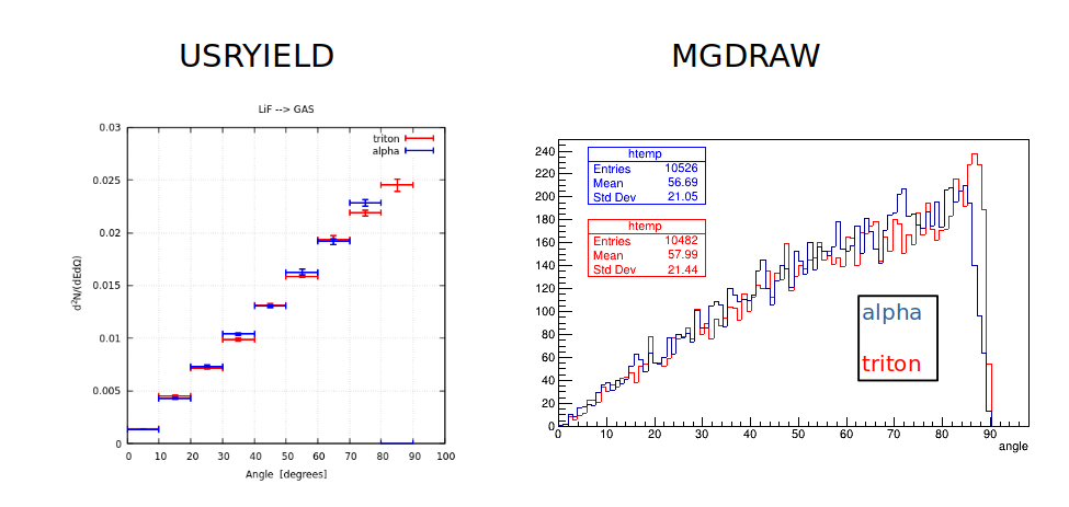
The USRYIELD is plotted in isolethargic way, while with boundary crossing estimator using MGDRAW I have a similar plot for alphas and tritons entering in the gas from the LiF converter…
My question is why there are more particles at large angles? Would it be isotropically distributed?
The angle is the polar angle in respect to the beam direction in Z.
So, in mgdraw I plotted the quantity Acoz(tzz) in degrees…
How this preference in large emission angles of the reaction products towards the gas could be explained?
Even before looking at your input, I would question the choice of isolethargic plotting of these spectra. You have nine linear angular bins, what reason is there to do so? Once you are no longer multiplying each histogram value with the average bin value (which increases linearly), the apparent linear increase will also largely disappear and take care of your observation. I would still expect a drop at high angles as the ions need to travel longer in the LiF layer and are more likely to stop before entering the gas.
(I assume you are treating your mgdraw scoring in the same way.)
We will in any case look at your input in detail and get back to you with further comments, but give this a shot in the meantime.
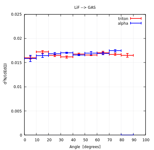
So it seems this the right representation of the particle yield…
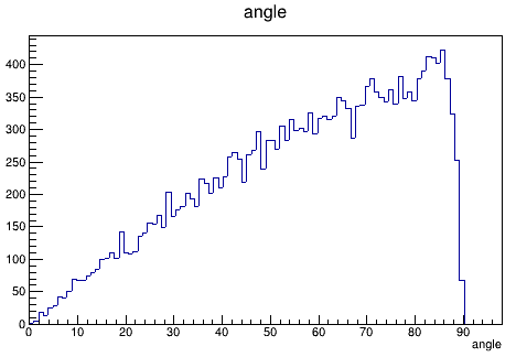
But why in mgdraw if:
the polar angle defined as ANGLE = 180.0*ACOS(CZTRCK)/PIPIPI ! 0 - 90 degrees
is different than the one indicated by USRYIELD that seems to be flat in all bins with a drop at high angles as you pointed out?
Great, we agree then that with the proper plotting the USRYIELD results make sense (although I find the dramatic collapse of the alphas in the last bin a bit suspicious).
The angle calculation in mgdraw seems correct, but how are you generating the plot? If you are processing the data in the same way as you were previously doing with USRYIELD it is not surprising to see the same result with the almost linear increase of the histogram.
As I mentioned, I will look into your input in detail and get back to you. Feel free to share the full mgdraw routine as well.
Sorry I accidentally deleted the post…
So, for a given neutron interaction point the direction the two capture fragments are emitted is isotropically distributed… mgdraw_1.f (17.7 KB)
From this subroutine only the bxdraw entry is relevant for this study…
If the polar angle is defined correctly as the arccosz my question is why at large angles there are more particles while with USRYIELD plotting in flair x vs y and not isolethargic, it is more or less flat…
Thanks so much for your time
(
Dear Andrea,
Please find attached the mgdraw I used… only the bxdraw entry is the relevant in this study.
I was thinking that the polar angle as the arccosz as given by FLUKA is equivalent with the polar angle introduced in USRYIELD. If it is correct, that implies that the initial direction of alphas or tritons inside the gas with respect of the neutron beam coincides with the polar angle BUT shows more particles at large angles where 0 degrees angle is when the direction of alphas / tritons is the same with the beam (parallel to Z axis)…
Let’s summarise. We agree that as far as the reaction is concerned, since the incoming thermal neutron carries very little momentum, the alpha and triton will basically share the Q-value among them inversely proportionally to their mass and be emitted in opposite directions with no particular preference (i.e. isotropically). This means that roughly equal numbers of particles will be emitted per unit solid angle - not per unit polar angle - and here lies the cause of the paradoxical results.
USRYIELD, being a mature, extensively tested and time-honoured scoring, of course accounts for this. Once we addressed the mistake of choosing a lethargy plot, we obtained a distribution in accordance with expectations. On the contrary, while the calculation of the polar angle in your mgdraw is correct, the post-processing is clearly not, most likely because you do not account for the fact that equal intervals in θ correspond to very unequal intervals in Ω, since Ω=2π(1-cosθ). E.g. the solid angle corresponding to θ between 0 and 10 deg is 0.095 sr, while between 80 and 90 deg (again a 10 deg interval in θ) it is 1.091 sr, therefore many more particles are emitted in this interval when emission is isotropic, and that is what you observe. Once you account for the Ω bin width Ω[i+1]-Ω[i]=cosθ[i+1]-cosθ[i], things will once more make sense.
Now, several more comments on your input follow. Many will have no bearing on your initial question, but some might.
You have set transport thresholds to 1 eV. This is way too low and meaningless. The lower limit is 1 keV, except of course for neutrons. Specifically for alphas, the minimum is 4 keV, although the documentation might (mis)lead you to believe that it is also 1 keV.
You are manually filling the Am field in many MATERIAL cards. This is not advisable and indeed blocked since the latest release. (Nice opportunity to update your installation to version 4-4.0.)
The use of LOW-MAT and LOW-NEUT cards makes no sense in the presence of LOW-PWXS. Note that pointwise neutron treatment is now the default since the latest release.
Not sure what that USERWEIG card is doing there, same for USRICALL.
IONTRANS and PHYSICS cards are also not needed here.
EMF ON is implicit for PRECISIOn DEFAULTs, no need to add it.
You define the gas with a 90:5 volume fraction of the two components. I just point it out in case it is unintended.
You may consider using a DETECT scoring in the gas for the energy deposition spectrum. Better than relying on the somewhat inflexible SCORE card.
The thickness of your LiF layer is 350 nm. That’s stretching the code slightly beyond its zone of comfort (μm scale and above).
In the mgdraw routine (just looking at the BXDRAW entry):
The condition IF(ETRACK.GT.AM(JTRACK)) is superfluous, as it checks whether the total energy is higher than the rest energy (one would hope so). A particle with zero kinetic energy will not enter the gas in the first place.
I am not sure what you are trying to accomplish with the IF(NTRACK.GT.0.AND.MTRACK.GT.0.) condition.
You may want to replace the somewhat archaic SNGL() with REAL() or, even better, define a FORMAT yourself, but as long as it works…
So, to conclude, there is a bit of clean-up work to do before running again. I hope the above helps, but do not hesitate to come back if something is still not clear after you have implemented these improvements.
I am really grateful for your help.
So just to clarify: If I would like to use mgdraw to calculate the “actual” emission angle of alphas/tritons inside the gas with respect of the beam direction, based on the recorded direction cosines in the boundary, the polar angle defined as ACOS(CZTRCK), is not the appropriate variable if it is plotted per equal polar angle bins. It should be corrected based on the solid angle effect…
Is there any direct formula as a function of the direction cosines that I could insert in the bxdraw entry to give the “actual” emission angle?
The “actual” emission angle of the particles is indeed the polar angle, there is no misunderstanding there. (Call it the lab emission angle if you will.) The issue arises when you try to make a histogram of the polar angles, expecting a roughly flat distribution, when in fact the distribution is only expected to be flat in terms of solid angle: equal number of particles per equal solid angle.
In other words: the polar angle bins of equal width (e.g. 10 deg) - that you legitimately and quite naturally choose - hide behind them solid angle bins of very different widths, increasing as the polar angle increases. That is why e.g. the bin from 50 to 60 deg contains more events than the one from 10 to 20 not despite but because of the isotropic emission. It it simply a larger basket for the particles to fall in and will therefore catch more of them.
So, the cause of the problem is not within the mgdraw routine, where you correctly determine the emission angle, but in the post-processing/plotting. You simply need to normalise the histogram bin contents by the corresponding bin width cosθ[i]-cosθ[i+1] (I mistakenly wrote cosθ[i+1]-cosθ[i] in the previous post), as you would do for any case when the bin width is not constant. To press the point further: if your first bin in a histogram is from 0 to 5, the next from 5 to 15 and the next from 15 to 50, what right would you have to expect a flat distribution if all values were equiprobable but you did not account for the different bin width?