biasing.inp (6.4 KB)
biasing.f (9.2 KB)
Dear Francesc,
Thank you. It worked. The source file is successfully built.
But, the results are zero at the lead surface. How to proceed further?
Kindly help.
With regards,
Jyoti
biasing.inp (6.4 KB)
biasing.f (9.2 KB)
Dear Francesc,
Thank you. It worked. The source file is successfully built.
But, the results are zero at the lead surface. How to proceed further?
Kindly help.
With regards,
Jyoti
Dear Jyoti,
Upon a quick glance, I see you start with ~1.17-1.33 MeV photons in several cm of stainless steel followed by ~30 cm of lead and are interested in the region afterwards. These photons (and the electromagnetic shower they set up) will struggle to make it out: it will be difficult to score anything in said region.
To convince yourself, try first scoring closer to the source region (closer to the axis of your cylindrical geometry) and witness how the e.g. the particle fluence quickly drops by orders of magnitude. This will give you a first feeling of what to expect. You may want to tweak / try more aggressive importance biasing (see next post), but after doing the exercise above, you will have an intuition on what to expect (essentially zero).
Cheers,
Cesc
Dear Jyoti,
in addition to @cesc’s excellent reply i would like to emphasize the usefulness of an USRBIN fluence scoring covering your whole geometry, which I was doing when I tested your input file:
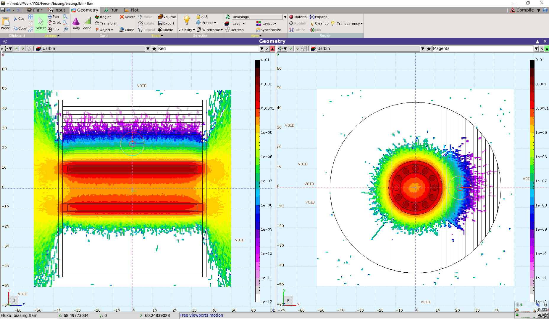
This will help you immensely to undersand what is happening in the simulation.
For example, I noticed that the most left cobalt rod is not emitting photons. If this is not intentional, then you need to check your source routine.
Furthermore I have some tips, how you can increase the effectiveness of the biasing:
I would use coaxial cylindrical layers in the shielding instead of the cut planes of on the right.
Your Cartesian scoring should be replaced with a R-Phi-Z one with only 1 angular bin, to take advantage of the cylindrical symmetry of your geometry.
It is clear that the biasing is not enough, you will need thinner layers. Unfortunately the maximum importance you can set for a region in 100000, which means you can double your last value again. However if you set the importance of all region to 0.0001. Starting with that you would be able to increase the number of layers by ~12, and still remain below the maximum 100000.
Cheers,
David
Dear David,
xzplot.pdf (132.7 KB)
xy plot.pdf (174.9 KB)
I have plotted photon fluence in x-y and x-z planes using Plot option. But, I am not getting the same plot as yours. Also, I am not able to plot it in Geometry Tab.
Kindly help.
With regards,
Jyoti
Dear Jyoti,
the difference may come from, that the standard plot averages the value along the 3rd axis. You need to set the Limits to only one layer of bins to match the plot on the Geometry Tab.
Please have a look at this presentation https://indico.cern.ch/event/956531/contributions/4020251/attachments/2120672/3569276/11_Flair_Advanced_2020_online.pdf from slide 19, especially slide 23. This will help you set up a layer showing USRBIN results in the Geometry Tab.
Cheers,
David
Dear David,
Thank you for the valuable suggestions. I am getting the results after giving importance of all region to 0.01. I have a small doubt in this case; since I gave all region importance to 0.01 and I am scoring the dose eq. at external surface of the geometry (here the importance is 0.01), do I need some normalization factor in the answer to calculate Dose eq./particle?
With regards,
Jyoti
Dear Jyoti,
It seems to me strange, that you get a result only with setting the region importance 0.01 everywhere, which negates the effect of biasing.
The increasing region importance through the shielding needs to be there, and the region outside the shielding has to be the same importance as the last layer.
FLUKA will take care of the correct normalization even if you are using biasing. No extra normalization is needed.
Cheers,
David
biasing.f (9.2 KB)
test2.inp (7.0 KB)
test2_21.bnn.lis (1.1 KB)
Dear David,
Thank you for the reply.
Sorry, I forgot to attach the input file. I have increased the region importance as I move away from the source. The result bin.lis file is attached. The last two values have large errors. (And, one cobalt rod is not emitting photons is intentional. )
For me the region outside the shielding is void. i) As you suggested, shall I give the importance of void same as the last layer (i.e., 41943.04).
ii) For any other case, If I would have given the blackbody to lastregion importance as 1, do we need to set void importance same as the last layer?
Dear Jyoti,
Yes the, you need to set the importance of VOID equal to the importance of the Boundary region. If you don’t do that the importance ratio between the two regions would be large, and FLUKA would kill most of the exiting particles. (The ratio is limited to 1/5 in FLUKA, i.e. maximum 80% of the particles can be killed)
This problem would remain if you set all the importance of all region to one in the first step. (This is the default values for regions where you don’t set the importance manually.)
In general it is a good practice to set the importances to one by hand regardless, since in collaborative work it is possible that importances are already set somewhere else, which could cause confusion.
In your case setting every region to 0.01 just simplifies the biasing setup, as you don’t need to specify the importances inside the shielding region by region.
Cheers,
David
biasing.f (9.2 KB)
test3.inp (7.2 KB)
analysis1.pdf (410.7 KB)
Dear David,
Thank you.
I have set the importance of scoring region and the boundary region same. I ran the file with usrbin as below:
R: 41 to 47 (3 bins)
phi: 12 bins
Z: -1 to 1
I got different values in phi: -30 to 0 and phi: 0 to 30 (the values should have been similar according to my geometry). There is a difference by a factor of E+02 in mSv/h. Similar difference is there in -180 to -150 and 150 to 180 bins. For phi: -30 to 0, the error is also large (analysis file attached). I don’t understand the reason. Kindly help.
To check whether I am doing some mistake in source co-ordinates in user subroutine, I simulated the values in air. The results are as expected, in the comparable phi bins-the values are similar (analysis file attached).
Thanks and Regards,
Jyoti
Dear Jyoti,
you need to take into account the error of the result as well. At one angle you have error around 5%, at the other around ~40%.
Take a look at slide 29 of this presentation:
According to this the result with the ~5% could be trusted, for the other angle you don’t have enough statistics.
To get better statistics, you need to run more primaries and/or you may need more aggressive biasing and/or increase the volume of your scoring along the z axis.
A fine scoring of covering your whole geometry should help to determine if you have good statistics, since it is easy to see it the colors change gradually or jumping erratically.
Cheers,
David
Calculations.pdf (1.1 MB) test4.inp (7.6 KB)
Dear David,
Thank you.
As you suggested:
However, my observations are not as expected:
I am not able to find the error in my input as the statistical errors are less (which can be trusted) but the results obtained seem to be incorrect.
Kindly suggest.
Thanks and Regards,
Jyoti
Dear Jyoti,
the main issue with your analysis that you have the order of numbers wrong. The ASCII files of USRBIN results are read line by line continuously, and the order of number are the following:
Also, the big errors in the “boundary” and “detector” region need to be addressed. They are caused by the unbiased photons leaving your geometry on the sides, when they are back scattered in air. They have significantly higher weight compared to the photons going through the shielding, so they contribute to the dose much more in value. But this happens very rarely, thus the statistics will be bad.
These two contribution is best to simulate separately:
Cheers,
David
Dear David,
Thank you so much for explaining so patiently.
It worked and my problem is solved.
Thanks again.
With regards,
Jyoti