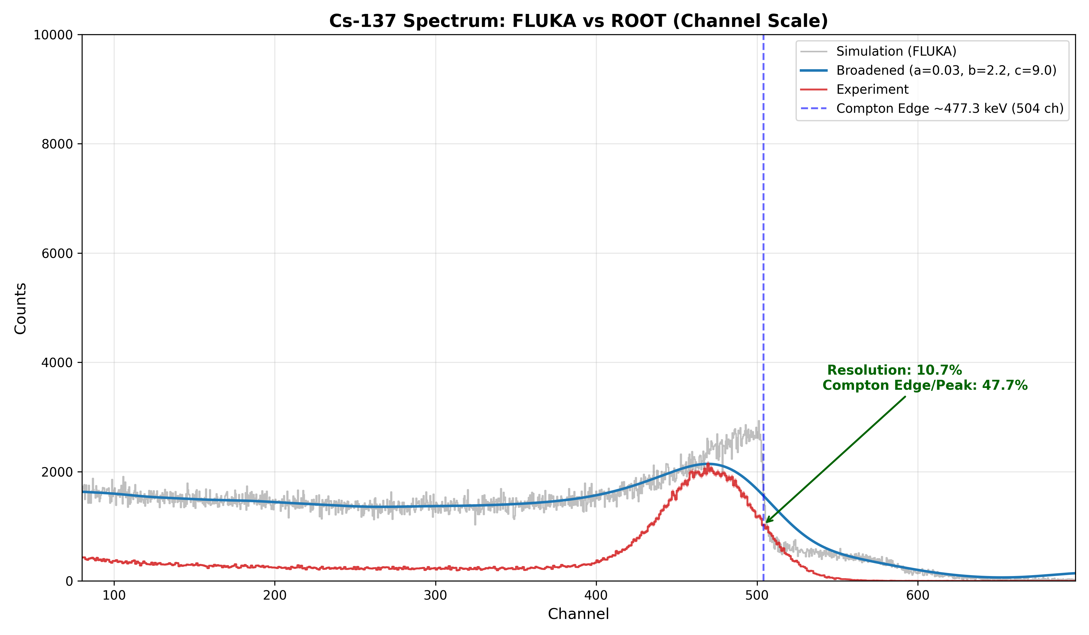
I am performing simulations for a two-detector coincidence measurement. The simulated energy spectrum disagrees with experimental data.
In experiment, we used CAEN DT5730 in coincidence mode with an 8 ns time window. For Cs‑137, this time gate strongly suppresses low-energy background. However, such background rejection is absent in my FLUKA simulation.
I enabled the coincidence flag on the DETECT card. I understand that the native DETECT coincidence only selects hits from the same primary history, without a configurable time cut. I suspect this is the root cause of the discrepancy.
Could you advise how to implement an 8 ns coincidence time filter between the two detectors in FLUKA?
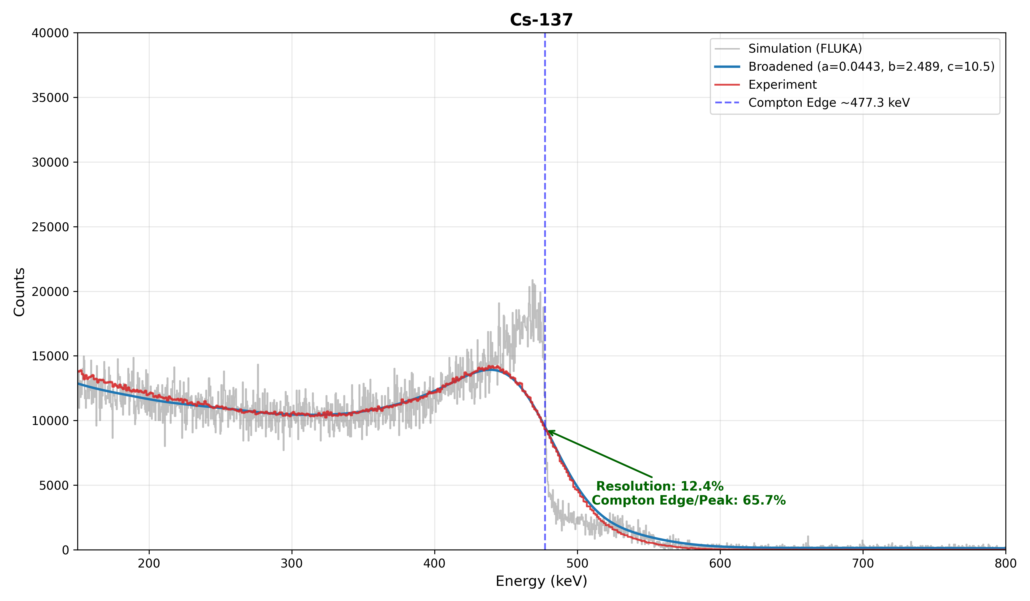
A figure comparing experimental and simulated spectra is attached.
We have had a look at your question and let me highlight the two following parts:
You intended to have a coincidence for the detectors in your DETECT card. However, the way you implemented it, you have not selected a trigger but all regions are summed up to a larger detector region. If you want to actually achieve a coincidence, you have to define the trigger region, which can be achieved by adding a minus in front of the region. It is well explained in the Example of the DETECT definition here 7.22.15. DETECT — FLUKA Manual
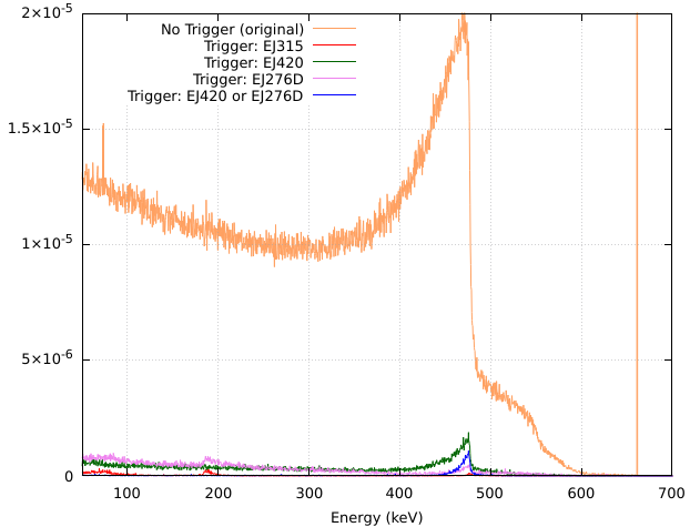
If you set region EJ420 as well as EJ276D as a trigger region, meaning you select the minus before the region, you will see that the low energy part is strongly suppressed and the curve is more similar to the data you see from your detector.
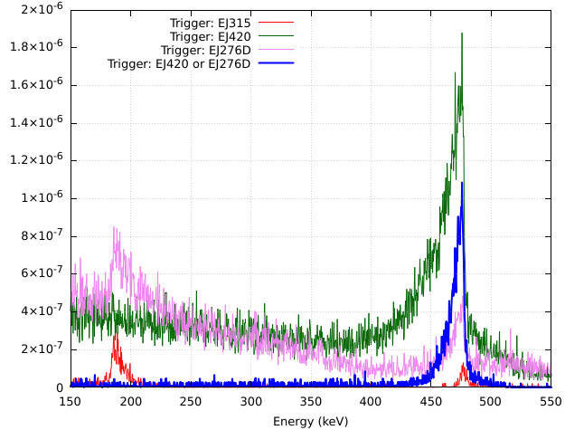
I have tried several combinations which is educative in understanding how selecting different trigger regions impact the eventual outcome. The two plots show the different Trigger settings in two scales:
Implementing a 8ns time cut is a delicate endeavor which is not required in your case. Your geometry ranges over around 10cm and no energy deposition takes place after 1ns from the Cs-137decay. Therefore, applying a 8ns time cut will be without any effect on the result.
I hope this clarifies your question and don’t hesitate to come back in case of further questions.
The main purpose of my simulation is to obtain the energy spectrum of EJ-315 in coincidence with the other detectors. If I want to record events where EJ-315 is in coincidence with either EJ-420 or EJ-276D (i.e., EJ-315 AND (EJ-420 OR EJ-276D)), should I put a minus sign in front of both EJ420 and EJ276D in the DETECT card?
Alternatively, should I use two separate DETECT cards, one for EJ-315 in coincidence with EJ-420, and the other for EJ-315 in coincidence with EJ-276D?
to obtain an energy spectrum of EJ-315 in coincidence with the other detectors, meaning being in coincidence with either EJ-420 or EJ-276D your DETECT card should look like that:
These settings produce the blue curve in the plot in the answer above. Keep in mind, you can adjust the other parameters to your needs.
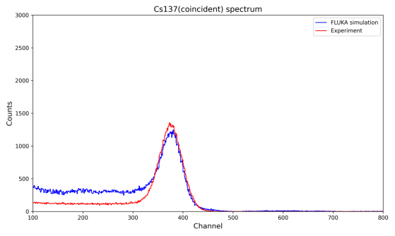
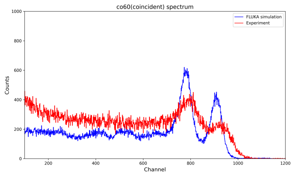
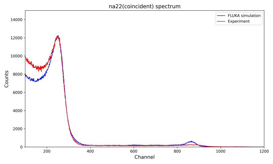
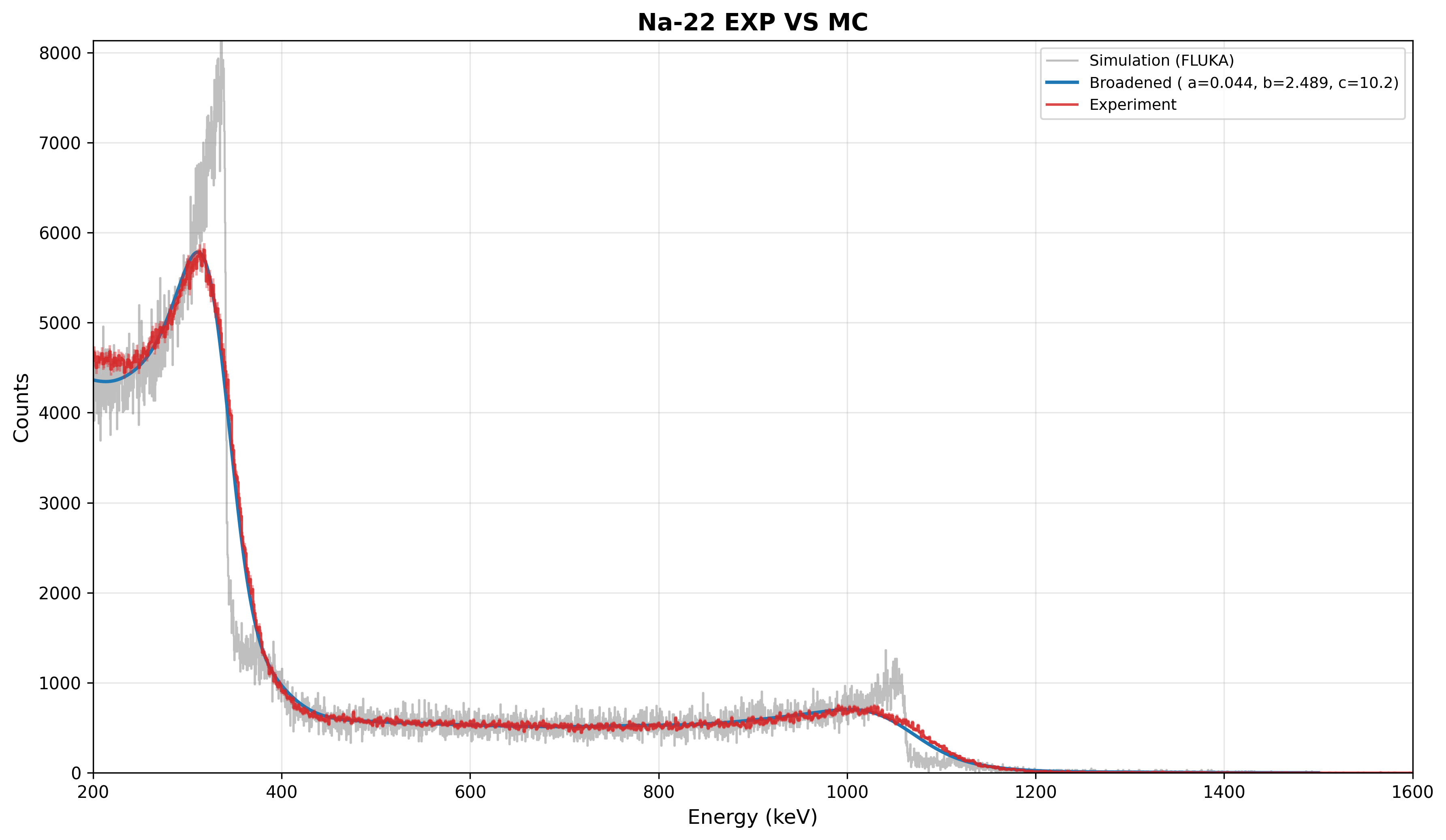
Thanks again for your help. I tried the approach with Na-22, Co-60 and Cs-137: the low-energy region agrees well with my data for all three, but the high-energy region of Na-22 and Co-60 shows clear discrepancies.
Could you give me a hint on what might cause this?
In general, the detector/source geometry, the detection mechanism, and the signal-processing electronics determine the shape of the spectrum, and it is difficult to tell the different factors apart in a coincidence spectrum. I recommend to compare simulations to singles spectra at low count rate (no dead time/pile-up) first to check whether they accurately reproduce the individual detectors’ response. In particular for coincidence measurements, it is important that the simulations reproduce not only the shape of the spectrum but also the absolute efficiency, since the coincidence count rate is a product of two efficiencies at (probably) two different energies.
The DT5730 module you are using is capable of recording singles and coincidence spectra at the same time, so you might already have singles spectra from the same runs.
Apart from these general considerations, I have some specific comments on your attached plots:
I would not conclude that the low-energy region agrees well with the data. For 137Cs, the simulation seems to overestimate the count rate in all channels below about 300, while for 60Co (22Na), it underestimates the count rate in all channels below about 700 (200), i.e. the behavior is the opposite. Are the spectra normalized to “counts per second”, and do they use the same binning? Or did you normalize them w.r.t the counts in one of the full-energy peaks (from the plots, I believe so)? The latter will not help you in deciding whether some part of the spectrum is over- or underestimated.
Barbara’s DETECT card uses Ecut = 0.0. Even if this is internally converted to FLUKA’s default value, your real detectors certainly have a higher threshold, and maybe even different ones. This option has the potential to reduce the low-energy background in the spectra.
In the 60Co spectrum, the simulation overestimates the detector resolution. The peaks in the experiment are broader. This might also explain the absence of the (1274+511)-keV peak in the experimental spectrum for 22Na, although one needs to admit that the 511-keV lineshape is in excellent agreement.
One more comment on the 22Na spectrum: As the simulation is set up right now, the positrons from the β+ decay are directly released into air because there is no region representing the source material. This means that the positrons are traveling too far. One would need to think more carefully about the implications for the coincidence spectra, but this is definitely not a realistic scenario.
Considering that we already talked about this …
… I suppose you took it into account here and the geometry you attached earlier just doesn’t show it.
Nevertheless, this even affects the β- decayers, especially 137Cs which relies on electrons to create coincidence events.
Thank you for your careful comments and reminder on source geometry.
Simulated EJ315 single spectra show similar features to experimental data. As a liquid scintillator, EJ315 shows Compton edges instead of full-energy peaks, since Compton scattering dominates over photoelectric absorption. Spectra are normalized on the falling slope of the Compton edge: ¹³⁷Cs (400–500), ⁶⁰Co (800–1200), ²²Na (240–400).
Source encapsulation is included for both ¹³⁷Cs and ²²Na, so positrons and β⁻ electrons slow down within the source matrix before entering air.
For the DETECT Ecut: my DT5730 trigger threshold is 36 mV (set in 300LSB), and its equivalent deposited energy is still unknown. My objective is minimum-χ² fitting on the Compton-edge slope for energy calibration and resolution modelling, not low-energy background rejection.
The FLUKA input and spectrum comparison plots are attached.
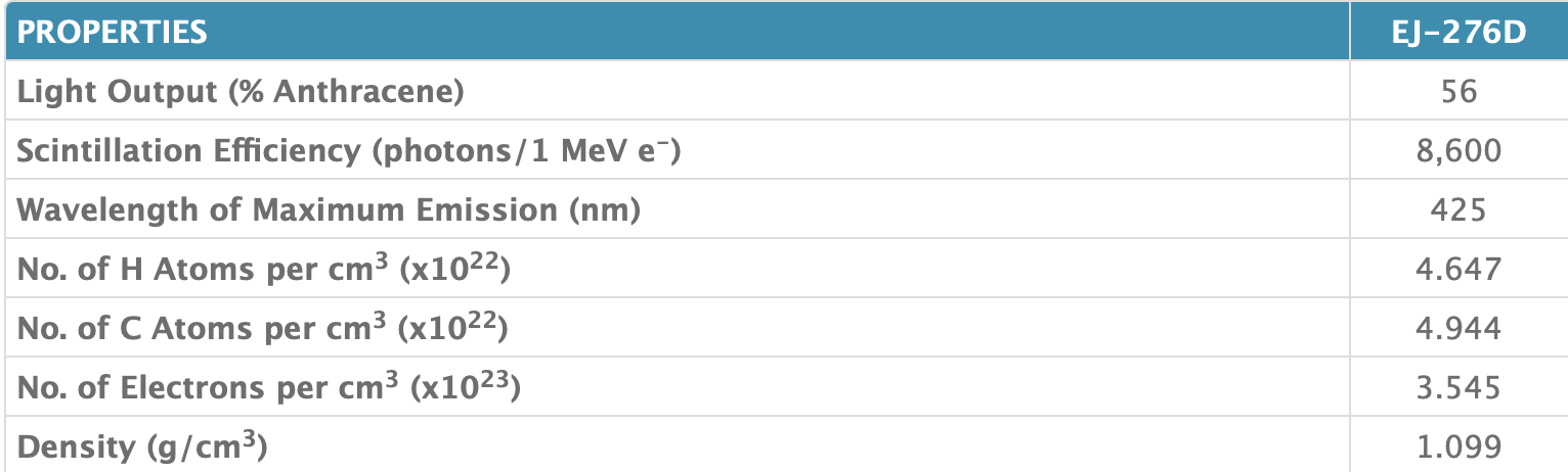
I am also wondering that whether the discrepancy seen in the coincidence EJ315 spectra could stem from an inaccurate material recipe used for EJ420. Eljen Technology does not provide the exact elemental or mass fractions of EJ420, while EJ276D has its atomic composition specified in the datasheet.
ej420: EJ-420 - Thermal Neutron Detector - Eljen Technology
As a liquid scintillator, EJ315 shows Compton edges instead of full-energy peaks, since Compton scattering dominates over photoelectric absorption.
Yes! Sorry for missing this in my reply. Replace “full-energy peak” by “Compton edge” everywhere.
Indeed, the shape of the singles spectra is in very good agreement with the data (as you already demonstrated in Inquiry on raddecay for Na22 beta-plus decay simulation ). This indicates that the material composition can’t be too far from reality.
The ultimate test would be a comparison of the simulated count rate (in some range of the spectrum, for example in the Compton-edge peaks) to the measured one, i.e. no normalization. You probably have information about the activity of the sources to do this check. However, I’d focus on the triggers first (see below).
For the DETECT Ecut: my DT5730 trigger threshold is 36 mV (set in 300LSB), and its equivalent deposited energy is still unknown.
I’d recommend to start with an educated guess for the threshold and then refine it. You know the voltage range of the digitizer (either 0 to 0.5 V or 0 to 2 V), the spectra indicate that Channel = 0 → Energy Deposition = 0 keV is a good assumption, and you can extrapolate the upper limit of the spectrum from the known Compton-edge energies. This should already give you a much better estimate of the threshold energy than the FLUKA default.
Maybe you can also read off the threshold in the singles spectra by comparing the low-energy cutoff channel to the Compton-edge channel.
To summarize my recommendations: Try to estimate the threshold first and see if this improves the coincidence spectra. If not, the efficiencies might be off. Dead time / signal pile up could also be investigated eventually. I am not sure how to detect symptoms of those effect in your detector type, however.
By the way: We might be deviating too much from the original question, but I’ll let some forum moderator advise us on what to do.