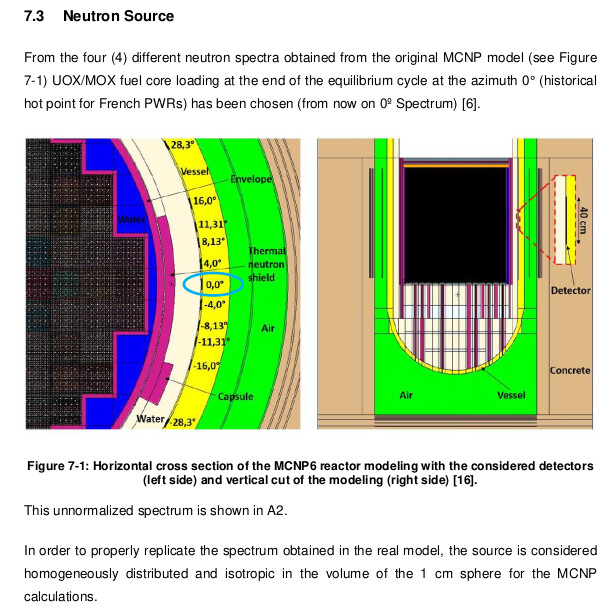
I am aware of a MCNP study where they calculate DPA taking into account the neutron flux spectrum and the intensity. In order to properly replicate the spectrum obtained in the real model, the source is considered there as homogeneously distributed and isotropic in the volume of the 1 cm sphere for the MCNP calculations.
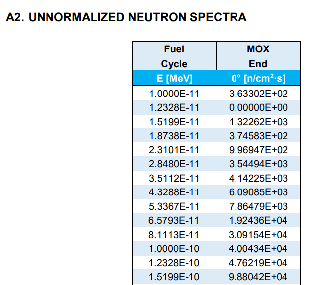
I was trying to calculate the DPA too using FLUKA. Thus, I used their unormalized neutron flux spectra (E[MeV], [n/cm^2*s]). The attached txt file is the one available BUT I add the 1st line at 0 as FLUKA requires when I am employing the source routine. There, for a volumetric source I used the SFLOOD function for an isotropic and uniform FLUENCE inside the sphere target as far as I understood from the MCNP evaluation.
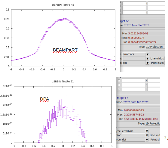
The DPA I get from the 73 FLUKA file in the Fe target is: 1.4170E-21
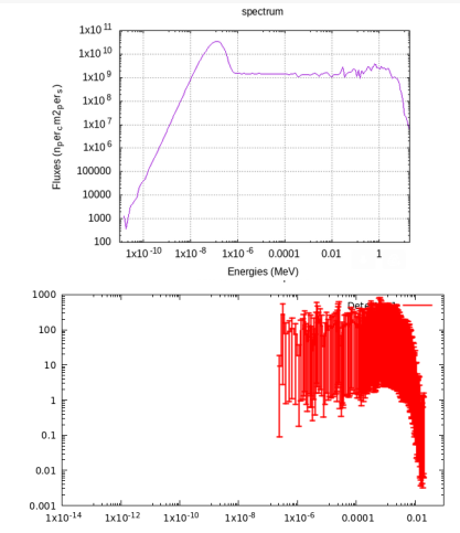
Multiplying it with Intensity and Running period gives a value ~ 50 greater that the estimated one with other codes as well. I am afraid there is a mistake in source routine I used… Also I wonder why the spectrum I am getting from FLUKA using USRTRACK, as you could see at the attached picture doesn’t have values at low energies like the original flux spectrum (top picture). - Was it a wrong sampling?
When I run with more statistics (x100) I have low energies values BUT not following the probability of the original spectrum.
I wonder whether you could have a look and let me know your suggestions…
thank you for your question.
Your implementation of the sampling from your histogram seems correct (calculation of the cumulative distribution and selection of the random energy interval) and the assignment of the primary coordinates and direction cosines using SFLOOD is also correct.
Assuming that the other settings and geometry are equal to the MCNP case, there are two possible issues. First you should add a second PART-THR card after the one you already have to transport neutrons down to thermal energies and overwrite the previous changes.
The second issue could be in the external file that you were given. You can quickly check it as well but the spectrum in your *.dat file is not normalized and, as such, cannot be used to sample the neutron energy in a healthy way. You can either normalize it offline and prepare another *dat file to be used, or you can normalize inside the IF (LFIRST) … THEN of the routine.
Before doing a run scoring DPA, I suggest you to put the target region to VACUUM and score the neutron fluence around the target (check the particle direction) and the neutron spectrum in the target: the latter should reproduce the input spectrum if properly sampled. In this way you will be confident that all is working as it should
In case you find any difficulty or have further questions do no hesitate to ask.
Cheers,
Davide
PS: I recommend you to switch to CERN FLUKA. Converting your source routine to the new format can be done quite easily and if you have any issue with the installation we will be ready to provide assistance
I had two other comments for your simulation. Unless you have a specific reason to do so, I would put the WHAT(2) of the SOURCE card (which you use to pass a value for the radius) to a value greater than the radius of the region where you score DPA (not lower and not equal since in the latter case particles would start at a boundary). Outside you have vacuum which will not influence the spectrum.
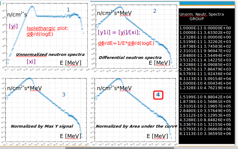
Note also that the spectrum that you have in the *dat file is iso-lethargic [dPhi/d(logE)]: if you plot the points without any manipulation, you see that the neutron slowing down region (1/E trend) is flat as it should in iso-lethargic spectra. It’s not wrong to use it (in the end any normalized histogram can be used), but mind that you are not sampling from the spectrum dPhi/dE.
I used it as it is without manipulation. The log in both axes in the pict at my 1st message is for visualization only. So, you suggest to normalize it by converting in probabilty cumulative dist? Now as it is, it is group energy arranged. How I should modify the hsource.f activating the “IF ( LFIRST ) THEN” part in order to normalize it and use it instead the 1st one?
Thanks a lot in advance
yes exactly. If you have doubts on how to implement that, please have a look at the files in this zip folder:example.zip (83.1 KB) Starting from the code that you had I added some lines to zero all the arrays before and to normalize the input spectra using your variable SUM. Let me know if that is not clear.
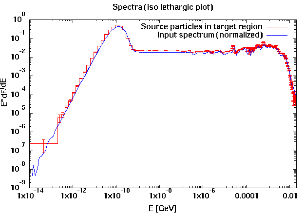
I converted the spectra that you gave me from iso-lethargic to simple differential (no magic behind it, is simply dPhi/dE = 1/E dPhi/d(logE) ) and normalized it. I have checked with the USRTRACK and it looks fine
Notice that the transport of low energy neutrons is performed in FLUKA by a multigroup algorithm with 260 groups: this is why you will not be able to reproduce the input spectrum with the same granularity.
Please give it a go and let us know if you have any other issue.
I am really grateful for your help. Now the simulation using Fe as the target material works nice, sampling from the low energy neutrons regime as well.
I just need to understand correctly the results in order to be able to compare with MCNP.
In my input I change the radius to 0.5 cm and the SOURCE input imposed value for the radius of the SFLOOD function to 0.501 and get the results as shown in the attached pict. The DPA (integrated) is: 4.5611E-23.
Should I use this DPA value x Intensity[n/s] x Operation time[s] in order to compare with MCNP? (or the maximum DPA ~ 2.2E-23 as it looks at the projection pict).
What is not too clear for me is their consideration as it is stated in the last 3 lines:
As far as I understood, If you need a spherical shell source and your target will be exposed inside that shell, then you can use SFLOOD function. If you need
isotropic distribution outside the spherical shell, then RACO function.
In this case, I used the SFLOOD function, but when its radius is greater for example 10 times more than the radius of the iron target, the DPA decreases ~100 factor. Also changing the radius of the Fe target results are changed too…
I wonder if the SFLOOD (and not the PACO) is the right approach…
apologies for the late reply.
The SFLOOD subroutine is the correct one to be used if you want a uniform and isotropic source within the sphere. The RACO subroutine returns 3 random numbers that can be interpreted as cosine directors of a random (isotropically ditributed) direction in space, it does not provide you a random position on the surface of the sphere as well.
Concerning your other question, the answer depends on what you need to compare in the end. As first point you should always look at the statistical uncertainty of your results: as a rule of thumb, if the relative uncertainty is greater or around 20%, the estimate hasn’t reached convergence so you should definitely run more primaries.
The second point is that the DPA is an intensive quantity. A USRBIN scoring will give you the number of displaced atoms per primary divided by the number of atoms in that bin: the result is then an average over the bin. If you use a region scoring you get an average over the region, not an integral: on this matter you can also change the 73 ASC in your input file to 73 BIN in this way you can merge results from different cycles and convert to ASCII the processed files (In the Run tab you have the Ascii button). It is up to you to identify the proper mesh resolution according to the information that you want to extract/compare: changing the bin size (hence the number of atoms in the bin) will lead to different result.
I have seen that you have correctly lowered the particles transport thresholds and added the MAT-PROP card with a threshold energy of 40 eV for Fe: just make sure that these settings are the same as the ones used in the other computation.
I hope this can be helpful. If you have any question please let us know.
Cheers,
Davide
PS: Of course, if you scale by source intensity (neutrons/s) times the irradiation time you would get the integrated value (over time), i.e bin averaged displacement per atoms.
Thanks so much for your clarifications concerning this study.
I tried to reproduce in MATLAB the differential plot by dividing each yi with the respective xi of the unnormalized neutron spectra and use this value on the plot-2 that gives the differential unnormalized spectra.
Thus, from the 1-plot (adding only the 1st line at 0: 1.0000E-11 0.00000E+00 at the initial table) I end up using the 4-plot (differential and normalized by Area under the curve) with the hsource.f routine I have attached at my 1st message without implementing any normalization inside the IF (LFIRST) … THEN part.
So, the 4-plot was the one I used for sampling with source routine invoking the SFLOOD function as you have pointed out as the correct approach.
For dpa calculation I used the value from the region binning. Multiplying it with intensity and operation time, I got exactly what MCNP gives!
I am very satisfied with this result. But the only thing that still puzzles me is that in the MCNP study it is stated that the neutrons table are: group energy plot and not lethargy. From literature I read that a group plot shows the number of neutrons in a given energy bin. Units for a flux/lethargy plot are n/cm2s, the same as group plots.The difference is that the group value is equal to the width of the energy bin (dE) times the differential flux where as the lethargy value is equal to the mid energy of the bin(E) times the differential flux.
As far as I understand, both ways of representing neutrons are very close each-other. Therefore, in my study -just to clarify it- the procedure I followed as it is stated out here using the 4-plot is still correct?
In addition, I end up using MATLAB because I couldn’t find a way to convert the flair plot in an ascii file with 2 columns of data… how we could have exported to numerical table of values like excell or ascii?
sorry for the late reply. I am very happy that the comparison turned out nice! I still think that the approach you followed so far is correct.
If you score spectra you will have the *tab.lis files which are tables that you can use to plot your results how you like. The same goes for USRBIN plots: once you make a plot, Flair generates a *dat file that you can use how you find convenient.
If instead you want to plot external data with Flair, you can do it as well by using the space reserved to gnuplot commands in the plot tab for example. If you go back to the *flair file that I have sent you as example, you fill see that for the 1D plot I have added the line plot 'NeutIDOM1.dat' us ($1*1E-3):($1*$2) w lines lt 1 lw 1 lc rgb 'blue't 'Input spectrum (normalized)'
In short this is the gnuplot command to plot the data in the file NeutIDOM1.dat using as x values the first column (I apply the scaling to get GeV) and as y values the energy times the differential fluence.
It takes a bit of practice maybe, but you can find online a lot of documentation and examples for gnuplot if you need them.