Hello everyone,
I want to determine the mass attenuation coefficient of a lead block using Fluka. In my research on the forum, I found the attached file uploaded by @youssef.allay and am using it. I have a question for you. First, what do the data I see in the lis files we obtained after the run mean? Are these I (or Io) values?
Hello again.
I wanted to make an update. After running the simulation, I went to the Data section on the flair. After processing, I returned to the Files section and obtained the attached files.
Thank you for your question. First, are you interested in the exact value of the mass attenuation of photons in lead? If so, I propose you have a look at the following post where this value is calculated for lead. I can provide some support with the user routines in case you are not familiar with them.
On the contrary, if you want to study the impact of certain lead geometry on the flux of photons, among others, you can use the approach of the file. Essentially, you obtain the output of the USRBDX card, showing the differential fluence of photons as a function of the energy and the solid angle in the interface between two regions. The tab file includes the angle-integrated fluence data as a function of the energy only. However, retrieving the mass attenuation from this may be not simple.
Please let me know if this is helpful.
Best regards,
Hello @msacrist ,
Thank you for answering. My main goal is to calculate mass and linear attenuation coefficient. Since writing my message, I have reviewed several examples. I placed my NaI detector and Aluminum material in the mgdraw example you sent. I aim to find values close to the results in the attached article. That’s why I imported all the geometry in this article into Fluka. Please let me ask you a few questions:
Can you give me some information on mgdraw? I have Fortran knowledge, although not at an advanced level. However, there are places where I get stuck. For example, does the 3 in the IREG=3 command take the 3rd place in the region section in Fluka? If so, should I choose Aluminum as the target or my detector? I’m not entirely clear here.
Normally, when we experiment in our laboratory, we follow the following procedure: First, we put only our point source (which is usually Co-60) in front of the detector and take measurements in this way for about 20 minutes, then we put our material in between and take measurements in this way. Thus, we determine the Io and I values. Then we apply the Beer-Lambert law. My question is: does the mgdraw routine also follow such a path?
In the article, the FEPE value was also calculated and the DETECT card was used. By adding this card, I created a mac_17_tab.lis file. But I don’t quite understand what column means in this file. Which one is the FEPE value? Or do I need to take action? I found various answers in the forum, but this part is unclear to me.
This question is somewhat related to the 3rd. Why do the error rates appear quite high when I plot the mac_17_tab.lis file in the Plot section? Is there any way to reduce this?
Thank you very much in advance, and sorry for so many questions.
Hello everyone,
I have been trying to determine the linear and mass reduction coefficient of Aluminum and Lead for a while. I created a geometry similar to this article (1-s2.0-S0272884220307987-main (1).pdf (1.5 MB)
). Measurements were made for glass there, but I want to do this for a lead block, not glass. The article states that the USRBDX card prints from RegLeft to the target for Io and from the target to RegRight for I. I implemented this, too.
However, I don’t know exactly what the results are.
i) What do the data in the sum.lis and tab.lis files I obtained after the USRBDX card mean?
ii) Which of these is I or Io?
ii)The results I obtained are a coefficient etc. Do I need to multiply by?
The linear attenuation coefficient is a value which is tabulated and can be accessed using mgdraw, as done in the post. This will provide you with the value used by FLUKA as a function of the energy and the material. Answering some of your questions about this option:
To use the mgdraw, you will have to recompile FLUKA with FLAIR, adding this user routine. Afterwards, you can run the simulation with the new executable.
IREG defines the region whose material will be used to obtain the coefficient. The region number is set based on the order in which you define the regions in the input file.
In the mgdraw file you can also set the range of energies of interest to obtain the coefficients.
On the contrary, if you want to simulate your experiment and compare it with your experimental results, then you can use something equivalent to your setup. The input file you have uploaded in your last post can serve as a good toy model. What you calculate with the two USRBDX cards is the flux [1/cm2/pp/GeV] entering the target from the left (Io) and the flux leaving the target from the right (I), respectively. Also, some answers:
The integrated flux over the solid angle can be found in the tab file.
USRBDX can output either the flux or the intensity over the surface. If you are interested in the flux, I suggest you use Phi1,LinE,LinTheta
You will obtain only one value since you request only one bin for the energy and solid angle. Also note that the Emax you define is lower than the primary energy, what means you will not include most of the particles.
You already add the normalisation factor (surface), but if you are interested in the ratio (I/Io) this should not play a role.
If you find high error bars, try using more primaries to improve the statistics. Many photons do not interact if the material is thin.
Dear @msacrist ,
Thank you very much for your tireless reply. Thanks to you, many points have become clear to me. Finally, wouldn’t it be disrespectful if I asked you to check whether I have made any mistakes in the attached file?
Here, I made void → target (21.bnx) for the Io value and target → void (22.bnx) for the I value. Is this the right choice?
As you said, I get the Tot resp (Part/cmq/pr) value in the sum.lis file. I read somewhere that I should normalize this value by 400 cm^2 * 0.001GeV * 100000. Is this true?
If I do this normalization;
My value in file 21.bnx: 2.4988151E-03 * 400 * 0.001 * 100000=99.952604
My value in file 22.bnx: 2.1179500E-03 * 400 * 0.001 * 100000=84.718
Hello @ysngyln ,
Thank you for the help. I know this site. However, my general goal is to find an accurate result for a material we know, like aluminum or lead, and to simulate the materials we want to produce.
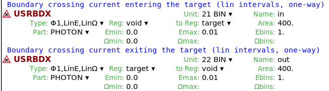
I propose you score photon flux, instead of photon current (they are not the same quantity, see the image).
The regions can work as they are defined currently.
Concerning the normalisation, it depends on your specific case. If you focus only on the flux ratio (I/Io), this is actually irrelevant. The value obtained in the tab file is [photon/cm2/pp/GeV]. You can multiply by the bin energy bounds (Emax-Emin, 0.01 GeV in your example) to obtain [photon/cm2/pp]. Note that you have defined the area of the surface as 400 cm2, but your target is actually much smaller. Lastly, if you are to compare only simulations among them, you may leave the ‘per primary’ normalisation. Should you want to compare a simulation to a real experiment, you may want to multiply it by the number of particles used in reality, by means of the activity of your source and irradiation time.
Dear @msacrist ,
Thank you. I made the corrections you mentioned, but I cannot get results similar to XCOM results. What could be the problem? Should I get the results from the tab file or the sum file?
Thank you, you can find my file attached. I am getting the Tot resp. value in the sum file. If I need to get the value from the tab file, how should I proceed? For example, the XCOM value of aluminum at 1 MeV is 0.06146 and its density is 2.7
Dear @gamze,
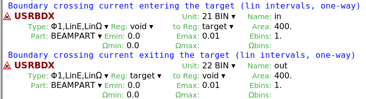
My apologies, the problem comes from the definition of the cards I offered. For your purposes of obtaining the attenuation coefficient, you shall score BEAMPART fluence, instead of PHOTON fluence (see picture)
BEAMPART refers to those primary particles (photons) which have not undergone any inelastic interaction while PHOTON includes every photon. In your example with 1 MeV photons, the dominant interaction is Compton scattering, where there is a product photon with lower energy. Hence, if you score PHOTON fluence over the whole energy range, you will obtain a higher value than the one retrieved with BEAMPART. However, please note that depending on your application, scoring PHOTON can be more representative of a real experiment. Using energy bins in USRBDX can be helpful to see how the energy of the photons is modified.
Thank you @msacrist . I will try again. So is the place where I read the values correct? Should I look at the sum file or the tab file? This part is still not completely clear to me.
Dear @gamze,
In the tab file you have, first, the differential fluence as a function of the energy [photon/cm2/GeV/pp] and after that the double differential fluence as a function of the energy and the solid angle [photon/cm2/GeV/sr/pp].
In the sum file, you have the detailed information for every bin and the cumulative result.
In your case, where there is only one bin, there is only one point of information. You can find it in the tab file twice and several times in the sum file. If you aim for [photon/cm2/pp], you shall multiply the single differential fluence [photon/cm2/GeV/pp] by the energy range (Emax-Emin, 0.01 GeV) or multiply the double differential fluence [photon/cm2/GeV/pp] by the energy range (0.01 GeV) and the solid angle range (2*pi).